Suppose we have a series of data points \(\{(\mathbf{x_1},y_1),(\mathbf{x_2},y_2),\ldots,(\mathbf{x_n},y_n)\}\) and there is some (unknown) relationship between \(\mathbf{x_i}\) and \(y_i\). Furthermore, the target variable \(y\) is constrained to be either a \(0\) or \(1\): a \(1\) label is considered a positive label, and a \(0\) label is considered a negative label.
We also have a black box that, given some input \(\mathbf{x_i}\), will produce as its output an estimate of \(y_i\), denoted \(\hat{y_i}\). This model is called a .
The question we will consider in these notes - without knowing any details of the classifier model - is how can we evaluate the performance of the classifier?
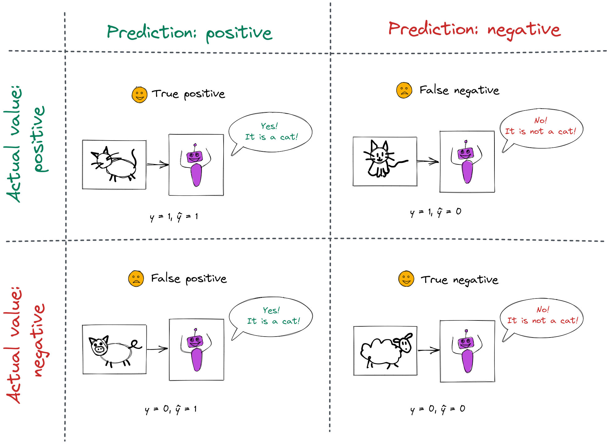
Consider a classifier model that is trained to identify cat photographs. Its output is \(\hat{y} = 1\) if it thinks the photograph is of a cat, and \(\hat{y} = 0\) otherwise.
For each prediction the classifier makes, there are four possible outcomes:

The number of true positive (TP) outcomes, true negative (TN) outcomes, false positive (FP) outcomes, and false negative (FN) outcomes, are often presented together in a confusion matrix:
| Actual \(\downarrow\) Pred. \(\rightarrow\) | 1 | 0 |
|---|---|---|
| 1 | TP | FN |
| 0 | FP | TN |
We may also define two more quantities:
The total population, P + N, is the total number of samples.
The most basic classifier performance metric is accuracy, defined as
\[ \frac{TP + TN}{TP + FP + TN + FN} = \frac{TP + TN}{P + N}\]
i.e., the portion of samples classified correctly.
However, accuracy is not always a useful metric. For example, imagine you are training a model to classify credit card transactions as fraudulent (\(1\)) or not fraudulent (\(0\)), but only 1% of transactions are fraudulent. A very basic classifier that always outputs \(0\) will have 99% accuracy! It is clear that accuracy is not a very useful metric here.
For a data set with highly imbalanced classes (\(P >> N\) or \(P << N\)), balanced accuracy is often a more appropriate metric:
\[ \frac{1}{2} \left( \frac{TP}{P} + \frac{TN}{N} \right) \]
Balanced accuracy gives the proportion of correct predictions in each class, averaged across classes.
In addition to the overall accuracy, a number of other metrics are used in various contexts. These are defined in terms of the four basic numbers described above: TP, FN, FP, TN.
\[ TPR = \frac{TP}{P} = \frac{TP}{TP + FN} = P(\hat{y}=1 | y = 1)\]
\[ TNR = \frac{TN}{N} = \frac{TN}{FP + TN} = P(\hat{y}=0 | y = 0)\]
\[ PPV = \frac{TP}{TP + FP} = P(y=1 | \hat{y} = 1)\]
\[ NPV = \frac{TN}{TN + FN} = P(y=0 | \hat{y} = 0)\]
\[ FPR = \frac{FP}{N} = \frac{FP}{FP+TN} = 1 - TNR = P(\hat{y}=1 | y = 0)\]
\[ FDR = \frac{FP}{FP+TP} = 1 - PPV = P(y = 0 | \hat{y} = 1)\]
\[ FNR = \frac{FN}{FN+TP} = 1 - TPR = P(\hat{y}=0 | y = 1)\]
\[ FOR = \frac{FN}{FN+TN} = 1 - NPV = P(y=1 | \hat{y} = 0)\]
These metrics are illustrated in the following table:

Another metric, known as F1 score, combines precision (\(\frac{TP}{TP + FP}\)) and recall (\(\frac{TP}{TP + FN}\)) in one metric:
\[F_1 = 2 \left( \frac{ \textrm{precision} \times \textrm{recall}}{\textrm{precision} + \textrm{recall}} \right)\]
The F1 score is also considered more appropriate than accuracy when there is a class imbalance. F1 score balances precision and recall: when both are similar in value, the F1 score will also be close to their value. However, if either precision or recall is lower, the F1 score will be “dragged down” by the lower metric.
The most appropriate choice of metric for evaluating a classifier depends on the context - for example, whether there is class imbalance, and what the relative cost of each type of error is.
It is trivial to build a classifier with no Type 1 error (no false positives) - if the classifier predicts a negative value for all samples, it will not produce any false positives. However, it also won’t produce any true positives! (Similarly, it is trivial to build a classifier with no Type 2 error, by predicting a positive value for all samples. This model will have no false negatives, but also no true negatives.)
We can often adjust the tradeoff between the FPR and TPR, depending on the cost of each type of error. Many classifiers are actually soft decision classifiers, which means that their output is a probability, \(P(y=1|\mathbf{x})\).
(This is in contrast to hard decision classifiers, whose output is a label, e.g. \(0\) or \(1\).)
We get a “hard” label from a “soft” classifier by setting a threshold \(t\), so that:
\[ \hat{y} = \begin{cases} 1, & P(y=1|\mathbf{x}) \geq t \\ 0, & P(y=1|\mathbf{x}) < t \end{cases} \]
By tuning this threshold we can adjust the tradeoff between FPR and TPR.
For example, consider our cat photo classifier from earlier, but suppose it is a soft decision classifier:
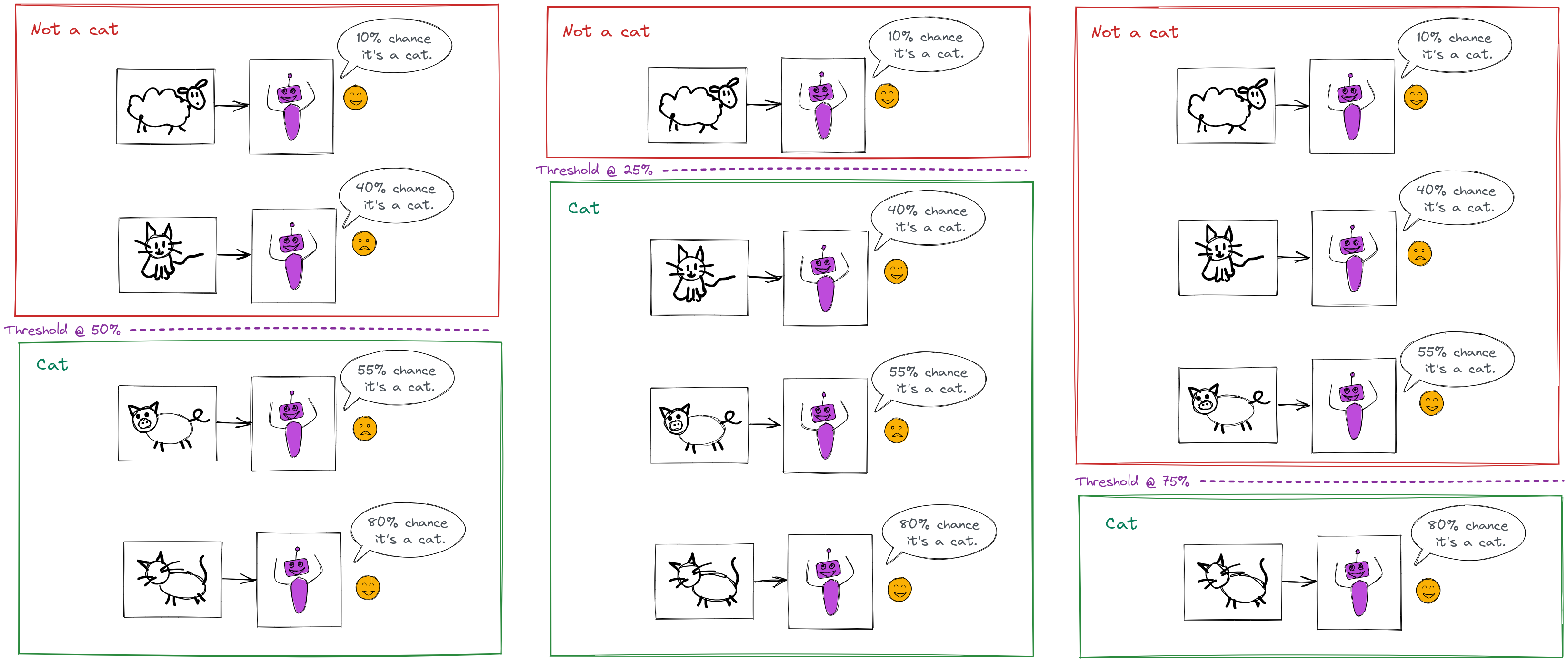
The performance of this classifier depends on where we set the threshold \(t\) for a positive prediction:
The label applied by the classifier depends on where we set the threshold, the error metrics above also depend on where we set the threshold. But, it’s useful to be able to evaluate the classifier performance in general, instead of for a specific threshold. We do this by plotting the TPR vs. FPR for every possible threshold, like in this plot:
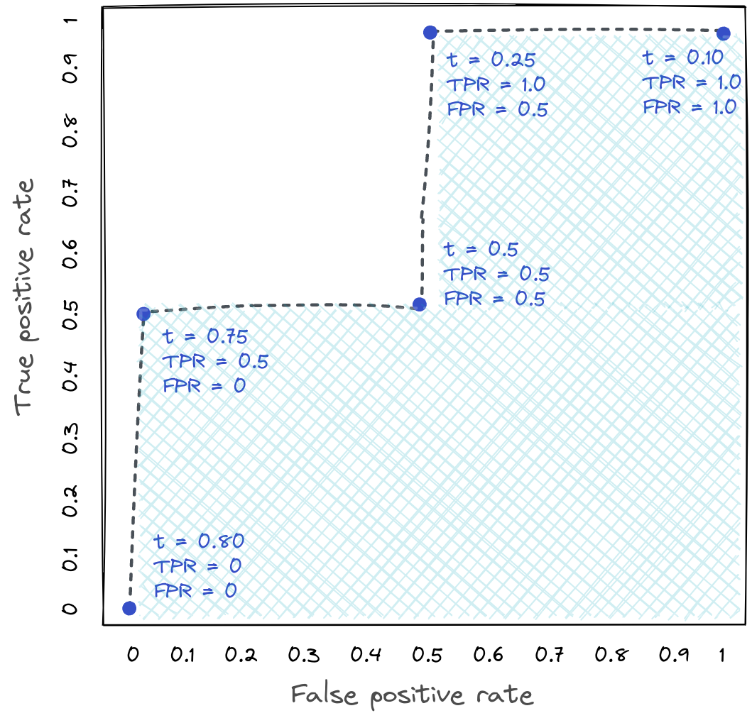
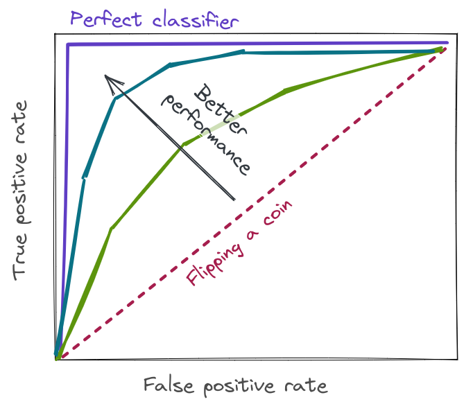
This plot is know as the ROC curve (receiver operating characteristic). The shaded area underneath the ROC curve is known as the AUC (area under the curve), and it is a classification-threshold-invariant way of evaluating the classifier performance.
A random classifier that doesn’t use any information about the problem will have an AUC of 0.5 (if both classes are equally prevalent in the data). A perfect classifier will have an AUC of 1. A typical machine learning model will have an AUC somewhere between the two, with a number closer to 1 being a better score.
So far, we have only discussed a binary classifier. For a multi-class classifier, the output variable is no longer restricted to \(0\) or \(1\); instead, we have \(y \in {1,2,\cdots,K}\) where \(K\) is the number of classes.
The same performance metrics apply to a multi-class classifier, with some minor modifications:
The error of a multi-class classifier can also be visualized using a confusion matrix, for example:
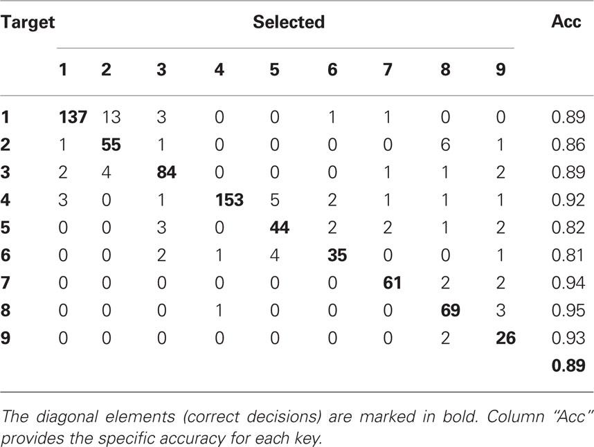
There is no universal rule for what makes a “good” classifier. It’s a common misconception that a “good” classifier should achieve some high accuracy e.g. 95%, 99%, etc. Yet, we have seen that even a very bad classifier will have high accuracy sometimes (if there is class imbalance). Meanwhile, for some very difficult problems, even a classifier with much lower accuracy may be useful (if it still has higher accuracy than any alternative solution). Finally, not all types of errors are equally “bad” - we may prefer a classifer that makes more errors overall but fewer “bad” errors, over one that has fewer overall errors but more of the “bad” type.
To decide whether a machine learning classifier is doing a “good job”, here are some helpful questions to ask yourself:
(You can check your answers to the first four questions here.)