5 Large model training
5.1 Preview
In this unit, we will introduce techniques for training large-scale machine learning models.
We will describe a selection of techniques to allow us to train models that would not otherwise fit in the memory of a single GPU, or to fit a larger batch in memory, such as:
- gradient accumulation
- reduced precision/mixed precision
- parameter efficient fine tuning (LoRA, QLoRA)
and we will also talk about strategies for distributed training across multiple GPUs:
- distributed data parallelism, which allows us to achieve a larger effective batch size,
- fully sharded data parallelism, which allows us to train models that might otherwise not fit into memory,
- and model parallelism, including tensor and pipeline parallelism, which distribute computation across GPUs
5.2 Review: backpropagation
This lesson is about training extremely large-scale models that require a lot of memory and compute - in practice, today, that means very large neural networks.
You may recall that neural networks are trained using backpropagation on a computational graph, where on the forward pass, each node stores intermediate values as the graph transforms the input.

Then to train it, we run a backward pass: each node computes a local derivative, and backpropagation accumulates those local gradients through the graph to produce parameter gradients efficiently.
The following images illustrate the operations performed at each node, in the forward pass and in the backward pass.
In the forward pass, we compute \(z_j\) at a node \(j\) as the weighted sum of inputs to the node:
\[z_j = \sum_i w_{j,i} u_{i}\]
Then, we apply an activation function \(g()\) to \(z_j\) to get the activation for node \(j\), \(u_j\).
In the backward pass, we compute the error term at node \(j\) using errors and weights from its output nodes, multiplied by a local derivative:
\[\delta_j = \sum_k \delta_k w_{k,j} g'_j(z_j)\]
then use this with cached inputs \(u_i\) to get parameter gradients, e.g. \(\frac{dL}{dw_{j,i}} = u_i \delta_j\).

Forward pass: use parameters from layer N-1 to N and activations from layer N-1 to compute
z_j (pre-activation) and then u_j (post-activation) at layer N; cache z_j and u_j for the backward pass.
delta_k from layer N+1, parameters from layer N to N+1, and cached z_j at layer N to compute delta_j; and multiply cached activations u_i from layer N-1 to compute parameter gradients at layer N.Considering that we are interested in training very large neural networks, let us consider what quantities we need to compute and what quantities we need to store in memory to perform these operations. Note that some of these quantities scale with parameters, and some scale with activations x batch size.
To compute the forward pass, at layer N, we need:
| Forward pass quantity at layer N | Why we need it | Scales with |
|---|---|---|
| Parameters from layer N-1 to N (weights and bias) | We use them with previous-layer activations to compute z_j at layer N. |
Number of parameters |
| Activations from layer N-1 (for each sample in the batch) | We combine these with layer parameters to compute z_j. |
Number of activations x batch size |
and we compute:
| Forward pass quantity at layer N | Scales with |
|---|---|
z_j (pre-activation at layer N, cached for backward pass) |
Number of activations x batch size |
u_j (post-activation at layer N, cached for backward pass) |
Number of activations x batch size |
To compute the backward pass, at layer N, we need:
| Backward pass quantity at layer N | Why we need it | Scales with |
|---|---|---|
delta_k from layer N+1 (for each sample in the batch) |
We use this to propagate error back to layer N. | Number of activations x batch size |
Parameters w_kj from layer N to N+1 |
We use these to map errors from layer N+1 back to node j at layer N. |
Number of parameters |
Cached z_j at layer N (for each sample in the batch) |
We use this to compute the local derivative at node j. |
Number of activations x batch size |
Cached activations u_i from layer N-1 (for each sample in the batch) |
We use these with delta_j to compute parameter gradients at layer N. |
Number of activations x batch size |
and we compute:
| Backward pass quantity at layer N | Scales with |
|---|---|
delta_j at layer N |
Number of activations x batch size |
Parameter gradients for layer N (for example, dL/dw_ji) |
Number of parameters |
| Optimizer state updates for layer N parameters | Number of parameters |
Let’s look a little more closely at optimizer state updates.
“Vanilla” stochastic gradient descent does not maintain any state:
for t in range(num_steps):
  dw = compute_grad(w)
  w -= lr * dw
But “vanilla” SGD doesn’t work very well on an unfriendly loss surface:
It may help to use momentum, but then we have to maintain a velocity vector (per-parameter):
v = 0
for t in range(num_steps):
  dw = compute_grad(w)
  v = gamma * v + dw
  w -= lr * v
or if we use something like AdaGrad/RMSProp, we need to maintain a vector of the second moment of the gradient (per-parameter):
grad_sq = 0
for t in range(num_steps):
  dw = compute_grad(w)
  grad_sq = gamma * grad_sq + (1 - gamma) * dw * dw
  w -= lr * dw / sqrt(grad_sq + epsilon)
and if we use Adam, then we need to maintain both - two state values per parameter:
moment1 = 0
moment2 = 0
for t in range(num_steps):
  dw = compute_grad(w)
  moment1 = b1 * moment1 + (1 - b1) * dw
  moment2 = b2 * moment2 + (1 - b2) * dw * dw
  moment1_unbias = moment1 / (1 - b1 ** t)
  moment2_unbias = moment2 / (1 - b2 ** t)
  w -= lr * moment1_unbias / sqrt(moment2_unbias + epsilon)
And, let’s observe that we are going to be especially concerned with quantities that scale with the number of parameters, since there are typically many parameters per activation:

We should also think about how long we need to retain each of these quantities:
- Training iterates layer-by-layer (forward from input to output, backward from output to input), and while operating at a layer N, we only need the quantities relevant to computation at that layer.
- During the forward pass, however, cached per-layer quantities accumulate from layer 1 to layer N, then backward pass consumes them from layer N back to layer 1 and can free them as it goes.
- And, all parameter gradients are needed for the optimizer step, so during the backward pass, we must keep the parameter gradients for each layer until the backward pass and optimizer step are complete.

Note that ML frameworks like PyTorch may still keep memory blocks reserved even after releasing the tensors saved in them.
5.3 Compute and memory bottlenecks
When we train a large model, each step has two kinds of limits. A compute bottleneck appears when we are mostly waiting for math operations to finish. A memory bottleneck appears when we are mostly waiting for data to be read, written, or moved.
We usually measure compute demand in FLOPs. Forward pass, backward pass, and optimizer updates all consume FLOPs, and backward pass tends to be especially expensive.
To meet the compute demands of training large neural networks, hardware acceleration (e.g. with GPUs) is essential. How did GPUs become so important for machine learning? GPUs were originally built for graphics workloads such as video games, where rendering repeatedly applies linear algebra operations to large arrays of values. They were also designed for high data parallelism: we run the same operation on many pixels, vertices, or fragments at once, which matches neural network training very well. (This is unlike multi-core CPUs, which are designed for task parallelism.)
In the early 2000s, GPUs became programmable for general-purpose workloads, and APIs from NVIDIA and others made it practical to run non-graphics operations on GPU hardware. This let ML frameworks map matrix-heavy training code onto hardware already optimized for massive parallel math.
Modern GPUs now often include tensor cores, which are dedicated matrix engines. Tensor cores are different from standard CUDA cores: CUDA cores are general arithmetic units, while tensor cores are specialized for matrix multiply-accumulate (the core operation in dot products, matrix multiplication, and convolutions) and can deliver much higher ML throughput for supported data types and tile sizes.
What about memory? For training, we need memory for parameters, gradients, optimizer state, and activations. There are multiple memory tiers. Inside a GPU, registers and shared memory are very fast but very small. GPU global memory is much larger, but slower than on-chip memory. Outside the GPU, host DRAM is larger again but slower. If tensors do not fit in the faster tiers, training can stall on data movement even when math units are idle. Under these conditions we may see low GPU utilization during training.
We saw that parameters, gradients, and optimizer state scale with number of parameters, while layer inputs/outputs and backpropagation error terms scale with activations x batch size. In convolutional models, activation size scales with spatial resolution, while in transformer-style models it scales with sequence length (and attention can increase this cost further).
Because these terms scale differently, the same model can hit different bottlenecks under different settings. For example, increasing batch size can make compute more efficient, but require more memory.
Broadly speaking, large convolutional networks are often more compute-limited, because convolutions can keep tensor cores busy with dense, regular math. Large language model training is often more memory-limited, because we must store very large parameter sets plus optimizer state and long-sequence activations. This is only a rule of thumb: either family can become compute-bound or memory-bound depending on model size, sequence/image resolution, hardware, and training settings.
5.4 Training large models on a single GPU
In this section, we will introduce strategies for training very large models - models with substantial compute or memory requirements - given a single GPU.
5.4.1 Batch size
Batch size is the number of examples we process together in one training step. If we process the entire dataset at once, that is full-batch gradient descent. In practice, we usually process smaller groups called mini-batches.
In either case, an epoch is a pass over the entire training set - we compute the gradient for each sample exactly once. In full-batch gradient descent, we make one parameter update per epoch; in mini-batch gradient descent, we make many smaller updates per epoch.


Why do we use larger batches when possible? Larger batches usually improve hardware utilization because the GPU can run more parallel work per step. They can also reduce gradient noise, since each gradient update averages over more examples.
Why can we not keep increasing batch size forever? The main limit is memory. Activations, temporary tensors, and some backward-pass buffers grow with batch size, so at some point we hit GPU memory limits. This is why batch size is often the first knob we tune when a run goes out of memory.
Batch size also changes optimization behavior. With very small batches, gradient estimates are noisy, which can help exploration but can also make training unstable. With very large batches, updates are less noisy and hardware throughput is often higher, but we may need to retune optimization settings, like learning rate.1,2
Furthermore, the number of epochs needed to reach a target accuracy is often a function of batch size. With smaller batch size, we do more weight updates per epoch. Because many datasets have redundant examples, those extra updates can help us reach good accuracy in fewer epochs.
A practical workflow is: start from a known-good baseline, increase batch size until we approach memory limits, then adjust optimizer settings while tracking both throughput and validation quality.
5.4.2 Gradient accumulation
Sometimes we want a specific effective batch size because we have a training recipe (optimizer, LR schedule, warmup, regularization) that is known to work at that batch scale.
Gradient accumulation lets us emulate a larger batch without storing activations for that full batch at once. We split a large logical batch into smaller micro-batches. For each micro-batch, we run forward pass (compute z_j, u_j) and backward pass (compute delta_j and parameter gradients such as dL/dw_{j,i}), then add those gradients to an accumulation buffer instead of stepping the optimizer immediately.
When a full batch does not fit in GPU memory, we keep per-micro-batch activation memory lower, but still get an update based on many examples before each optimizer step.
The effective batch size is:
\[\text{effective batch size} = \text{micro-batch size} \times \text{accumulation steps}\]
(When we later move to data parallel training, we multiply by number of GPU devices as well.) So if we use micro-batch size 8, accumulation steps 4, and one GPU worker, the effective batch size is 32. That means that we step the optimizer after 32 samples.

The tradeoff is: with gradient accumulation, we need less memory to work with the same effective batch size. But training can take a little more time, because we run several smaller forward and backward passes before each weight update.
5.4.3 Reduced precision
Floating point numbers can be stored in different formats with different numbers of bits. A floating point value is typically split into a sign bit, exponent bits (which control numeric range), and mantissa bits (which control precision).

Formats like FP32, FP16, and BF16 trade range and precision differently, so choosing a lower-precision format can reduce memory use and increase speed, but also changes how accurately very small or very large values are represented. FP32 is the most numerically robust of these three, but it uses the most memory and is often slower for matrix-heavy training workloads. FP16 uses half the storage of FP32 and can be very fast, but its smaller exponent range makes underflow and overflow more likely. BF16 also uses half the storage of FP32, but keeps a wider exponent range than FP16, so it is often more stable for training while still giving major speed and memory benefits.
On older GPUs, BF16 support may be limited. But modern data center GPUs support FP16 and BF16, and many training stacks are optimized for these types, e.g. has fast tensor core instructions for FP16 and BF16 matrix operations.
We don’t get anything for free, though. Reduced precision saves memory, and can make compute faster (because more data fits in fast memory, and because GPUs can compute matrix operations on reduced precision matrices much faster). It can also make compute faster just because the memory savings allow for a larger batch size! But reduced precision can hurt training quality, if numerical errors become too large.
5.4.4 Mixed precision
If weights/gradients are kept only in low precision, tiny but important updates can get rounded away. Over many steps, that can hurt convergence.
To address this, mixed precision combines low-precision and higher-precision arithmetic in the same training step. In the most common types of mixed precision training (fp16-mixed or bf16-mixed), we store full precision (FP32) model weights and optimizer state. But before heavy operations, we convert to lower precision and perform the operation in lower precision (FP16 or BF16). This is in contrast to e.g. fp16-true or bf16-true, where the parameters themselves are stored in lower precision.

Note that we need scaling in this flow. In FP16 training, very small gradient values can underflow to zero, which means we lose useful learning signal. Loss scaling addresses this by temporarily multiplying the loss before backpropagation so gradients are represented in a safer numeric range. Before applying updates, we remove the scale so the final parameter update has the correct magnitude.
Newer GPUs may support Transformer Engine integration (transformer-engine or transformer-engine-float16 precision), where precision is chosen dynamically for transformer layers: FP8 is used where it is not likely to harm numerical stability or model quality, and higher precision (BF16 or FP16) is kept for sensitive operations.
For models with a very large number of parameters, mixed precision training doesn’t save nearly as much memory as “true” reduced precision, because it still needs enough memory to keep the parameters and optimizer state in the higher precision. But it does give us memory savings for the quantities that scale with activations x batch size - pre-activations z, activations u, backprop error terms delta - which may be kept in reduced precision. The compute throughput may improve (because more data fits in fast memory, and because GPUs can compute matrix operations on reduced precision matrices much faster), but converting between high precision and reduced precision can also hurt throughput. Like reduced precision, training quality may be affected, but the impact is partially mitigated by keeping master weights and gradients in FP32.
5.4.5 Reduce optimizer memory
As we saw in the backpropagation review, optimizer state is part of training memory, and it scales with number of parameters. For large models with many parameters, this can become one of the largest memory terms.
A less-stateful optimizer is an optimizer that keeps fewer extra values per parameter. SGD keeps little or no extra state, momentum SGD keeps one extra state tensor (velocity), and Adam or AdamW keep two extra state tensors (first and second moments). This is why optimizer choice affects memory even when the model architecture is unchanged.
Reducing optimizer state can reduce memory pressure, but it can also change optimization behavior. In some workloads, this can slow convergence or reduce final quality.
We could also apply some of the other techniques described in this chapter (reduced precision, CPU offload) to the optimizer state. For example, we can keep an Adam-like optimizer but store optimizer state in lower precision, for example with 8-bit states in bnb.optim.Adam8bit from bitsandbytes. This can reduce memory substantially while preserving much of Adam-style behavior, but at the cost of some precision and potentially training quality. Or we can keep optimizer state on CPU memory instead of GPU memory (DeepSpeedCPUAdam from DeepSpeed), trading off memory for compute speed.
5.4.6 CPU offload
GPU memory is often the hard limit on the maximum model size we can train, while CPU RAM is usually much larger. If we want to train a very large model on a GPU with limited VRAM, we can move some training state (optimizer state, parameters, gradients, and sometimes activations) from GPU memory to CPU memory, and move it back to GPU memory when needed.
The tradeoff is transfer overhead: moving these values over PCIe/NVLink can reduce throughput and GPU utilization, so it is typically a “last resort” type of intervention. But this can still be worthwhile when offload is the difference between “model does not fit” and “model trains successfully.”
5.4.7 Activation checkpointing
In standard training, the forward pass stores many intermediate activations so the backward pass can use them later. Activation checkpointing changes this: we save only some activations (“checkpoints”), and during backward pass we recompute the missing ones when needed.
Why do we do this? Activation memory grows as we increase model size, input size, or batch size. If we run out of GPU memory because of activations, checkpointing can make training fit without changing the model itself.
The tradeoff is straightforward: we need less memory, but compute becomes slower, because we repeat part of the forward computation during backward pass. So each training step may be slower, but we can train models or batch sizes that otherwise would not fit.
5.4.8 Parameter efficient fine tuning
When we fine tune a pretrained model for a new task, we usually adjust only a focused part of its behavior, not rebuild everything it already knows. In many cases, this means we do not need a completely new set of full weight updates for every layer. Parameter efficient fine tuning uses this idea: instead of learning a full dense update for every weight matrix, we learn a much smaller update structure that approximates the same effect on layer outputs.
In LoRA (Low Rank Adaptation), we approximate the layer outputs produced by W + (full weight update) with W + AB, where A and B are low-rank factors and r is the rank. (W is kept frozen.) Because r is much smaller than the full matrix dimensions, we train far fewer parameters while keeping nearly the same mapping from layer inputs to layer outputs.3
QLoRA (Quantized LoRA) takes this one step further: it keeps the pretrained base weights in quantized form (for example 4-bit) and still trains only the low-rank adapters. This reduces memory much more than LoRA alone, because the largest tensor in memory (the frozen base model weights) is compressed. Why is this usually acceptable? The quantization error in the frozen base weights is often small enough that the trainable LoRA adapters can compensate for it during fine tuning, so we still get good task performance with much lower memory use.4


LoRA and QLoRA greatly reduce trainable parameter count, which in turn reduces memory use and makes compute faster. This makes fine tuning much more accessible on limited hardware. But they also constrain how much we can change model behavior, so for some tasks they may underperform full fine tuning, especially as we reduce r. QLoRA adds even more memory savings, but quantization can affect training quality and can also add compute overhead from quantization/dequantization.
5.4.9 Summary
| Technique | Main benefit(s) | What we pay |
|---|---|---|
| Larger batch size | Better hardware utilization for compute; less noisy gradient estimates | Requires more memory; may need to re-tune optimizer |
| Smaller batch size | Needs less memory; can sometimes help optimization | Noisier gradients; usually lower hardware utilization for compute |
| Gradient accumulation | Larger effective batch without increasing memory as much | More forward/backward passes per optimizer step means slower time per effective batch |
Reduced precision (fp16/bf16/etc.) |
Lower memory use; potentially faster compute | Possible numerical instability or quality loss |
| Mixed precision | Some of the speed benefits and better stability than true low-precision training | Not as much memory benefit as true low-precision training; casting/scaling may reduce compute throughput; still some potential for quality loss |
| Less-stateful optimizer | Needs less memory | Possible convergence/quality tradeoffs |
| CPU offload | Permits training models that wouldn’t fit in GPU memory | Transfer overhead on PCIe/NVLink; lower compute throughput and GPU utilization |
| Activation checkpointing | Needs less memory | Extra recomputation in backward pass; slower training |
| PEFT (LoRA/QLoRA) | Many fewer trainable parameters; lower memory and often faster fine tuning | May underperform full fine tuning on some tasks; QLoRA adds quantization overhead |
5.5 Training large models on multiple GPUs
So far, we focused on techniques that make one GPU go further. But for some model sizes and training-time targets, single-GPU optimization is not enough, and we need to split work across multiple GPUs. In this next section, we will look at strategies for multi-GPU training.
5.5.1 Collectives
To understand multi-GPU training, we need a core building block: collective communication. A collective is not specific to GPUs or model training; it is a general distributed-computing primitive used whenever many workers need to exchange and combine data in a coordinated way. These operations are the plumbing of multi-GPU training, because they allow GPUs to exchange enough information so the full training step stays consistent.
In distributed computing, there are four fundamental collectives that appear often across systems:

These four primitives are:
broadcast: one worker sends the same data block to all workers.scatter: one worker splits data into pieces and sends different pieces to different workers.reduce: all workers send data blocks to one destination worker, which combines them (for example, by summing).gather: all workers send their local data block to one destination worker, which collects all pieces.
They can be combined to produce aggregate operations. For example, all-reduce combines values from all workers and returns the combined result to every worker, and can be achieved by a reduce followed by a broadcast.

Or, all-gather collects local pieces from all workers and returns the full combined collection to every worker, and can be achieved by a gather followed by a broadcast.
For multi-GPU neural network training, we will need to use all-reduce very frequently. Historically, a major contribution that made multi-GPU (and multi-node) training much more scalable was ring all-reduce, which substantially reduces communication bottlenecks. So, let’s take a moment to understand how and why it works.
The figure below shows a “distributed data parallelism” (DDP) setting. Initially, each GPU gets an entire copy of the model, and a shard of data. It works locally to get gradients for its shard of data. Then, we need an all-reduce to average those updates so every GPU applies the same synchronized update.

We know that we can implement all-reduce with a reduce followed by a broadcast:


In reduce, each worker sends its local gradients to one destination worker, which combines them. In broadcast, that destination worker sends the combined gradients back out to all workers, so they can all apply the same weight updates. But note that communication volume scales with both tensor size and number of workers: for a tensor of size K across N workers, this pattern moves about 2(N-1)K total data, and the destination worker becomes a communication bottleneck because it must receive and send N-1 copies.
There’s another way to do all-reduce. Initially, each worker holds a gradient tensor computed on a subset of samples, but for all of the model’s parameters. Suppose we split that into shards, corresponding to different subsets of the model’s parameters. Then we do a reduce-scatter so each worker holds one reduced shard (gradient for a subset of the model’s parameters, but aggregated across all the data samples used by all the workers). Then we do an all-gather so every worker receives all reduced shards. The figure below shows this decomposition.

Compared with a single-destination reduce + broadcast, if we arrange the GPUs in a ring topology:

then this pattern distributes communication more evenly across workers and avoids one central bottleneck. Let’s see why by working through a single all-reduce, step-by-step:

We can see that unlike reduce + broadcast, which creates a central bottleneck, ring all-reduce spreads communication across workers: each worker sends and receives 2(N-1)K/N data for a tensor of size K across N workers. The per-worker communication stays roughly constant instead of growing linearly with N.
5.5.2 DDP
Distributed Data Parallelism (DDP) keeps one full copy of the model on each GPU. Each GPU receives a different shard of the batch, runs forward and backward locally, and then all GPUs synchronize gradients with all-reduce before applying the optimizer step.5

DDP works by allowing us to have a larger effective batch size, since gradients are accumulated across the shards of data held by each device before the optimizer step. With DDP, the effective batch size grows with device count:
\[\text{effective batch size} = \text{per-GPU batch size} \times \text{number of GPUs} \times \text{accumulation steps}\]
So if per-GPU batch size is 8, we use 4 GPUs, and accumulation steps is 1, the effective batch size is 32.
DDP scales well because most compute still happens locally on each GPU, and the main synchronized data is gradients. For compute-limited runs, this often gives strong throughput gains compared with a single-GPU run.
In practice, each step is limited by whichever is slower: local compute or inter-GPU communication. The main communication bottleneck is during gradient synchronization. As model size and number of workers grow, all-reduce can dominate the step time.
Note that DDP replicates model parameters and optimizer state on every GPU. This improves throughput, but it does not reduce per-GPU model-memory requirements for model states (parameters, gradients, optimizer state). The main memory win is that global effective batch size can be larger because each GPU only holds its local per-GPU micro-batch activations.
5.5.3 FSDP
But, why stop there? With ring all-reduce making exchange of values more scalable, maybe we can divide more than just input data between GPUs. Fully Sharded Data Parallelism (FSDP) is a distributed training strategy where parameters, gradients, and optimizer state are partitioned across GPUs instead of fully copied on every GPU.6

Why does this matter? DDP improves throughput, but still replicates full model states per GPU, so per-GPU model memory remains a hard limit. We “save” on memory for quantities that scale with activations x batch size, but not for quantities that scale with number of parameters. FSDP addresses that limit directly by also dividing across workers the quantities that scale with number of parameters, so each worker only needs to keep a fraction of them. This allows us to train models that would not fit under standard DDP.
With FSDP, we still need the quantities mentioned above to compute the forward pass/backward pass for Layer N. But we will get these quantities “just in time” when we are “at” Layer N, and then release them again. Here’s the outline:

In the forward pass:
- Each worker keeps only its local shard of parameters “at rest”.
- Before computing a layer, workers exchange shards so each worker can reconstruct the full parameters needed for that layer (
all-gather). - Each worker runs the forward computation for the layer on its local data shard.
- After the layer forward pass is done, full-parameter buffers can be released, and only the cached activations and sharded state remain.
In the backward pass:
- Before a layer’s backward pass, each worker all-gathers that layer’s parameter shards so it has the full parameters at that layer.
- Using those full parameters plus its own cached forward activations for that layer (from its local mini-batch shard), each worker computes local gradients.
- Those local gradients are then reduce-scattered: gradients are summed across workers and split. Every worker ends up with gradients for its own parameter shard, computed from every worker’s data shard.
- Temporary full-parameter buffers can be freed after use.
After all layers finish the backward pass, each worker runs the optimizer step on its local parameter shard.
For FSDP, ideally we should have enough memory to keep about 2 layers’ worth of parameters: the full weights of the layer currently being computed, and the full weights of the next layer, so that we can pre-fetch them during computation. This helps hide communication latency, since the communication happens in the background while we are anyway busy with computation:

ZeRO7 popularized the idea of sharding in stages, depending on model size and memory size. Using the notation from the ZeRO paper (Psi = parameter memory, K = optimizer-state multiplier, N_d = data-parallel workers), per-worker model-state memory is:
| Strategy | What is sharded across workers | Per-worker memory from ZeRO paper | Example from paper (K=12, Psi=7.5B, N_d=64) |
|---|---|---|---|
| Baseline (DDP) | Nothing | (2 + 2 + K) * Psi |
120 GB |
ZeRO-1 (P_os) |
Optimizer state only | 2Psi + 2Psi + (K*Psi)/N_d |
31.4 GB |
ZeRO-2 (P_os+g) |
Optimizer state + gradients | 2Psi + ((2+K)*Psi)/N_d |
16.6 GB |
ZeRO-3 (P_os+g+p) |
Optimizer state + gradients + parameters | ((2+2+K)*Psi)/N_d |
1.9 GB |
As we move from ZeRO-1 to ZeRO-3, memory per worker drops, but communication and coordination requirements increase.
5.5.4 Tensor parallelism
Both distributed data parallelism and fully sharded data parallelism are considered types of data parallelism: every worker does all the computations (a complete forward pass and backward pass over the network), but on its own small chunk of data. However, it is also possible to divide the computation among workers, an approach known as model parallelism. Tensor parallelism (this subsection) and pipeline parallelism (next subsection) are both types of model parallelism.
In tensor parallelism, we split one layer’s math across workers. For example, suppose one layer computes:
\[ Z = XW, \qquad U = \mathrm{ReLU}(Z) \]
where \(X\) is the input activation matrix and \(W\) is a very large weight matrix. If we split \(W\) by columns across 2 GPUs:
\[ W = [W_0, W_1] \]
then GPU 0 computes:
\[ Z_0 = XW_0 \]
and GPU 1 computes:
\[ Z_1 = XW_1 \]
Together they form:
\[ Z = [Z_0, Z_1], \qquad U = \mathrm{ReLU}(Z) \]
This lets us train layers that are too large to fit on a single GPU by sharding their parameters across GPUs and exchanging only the needed activations/gradient information during computation.
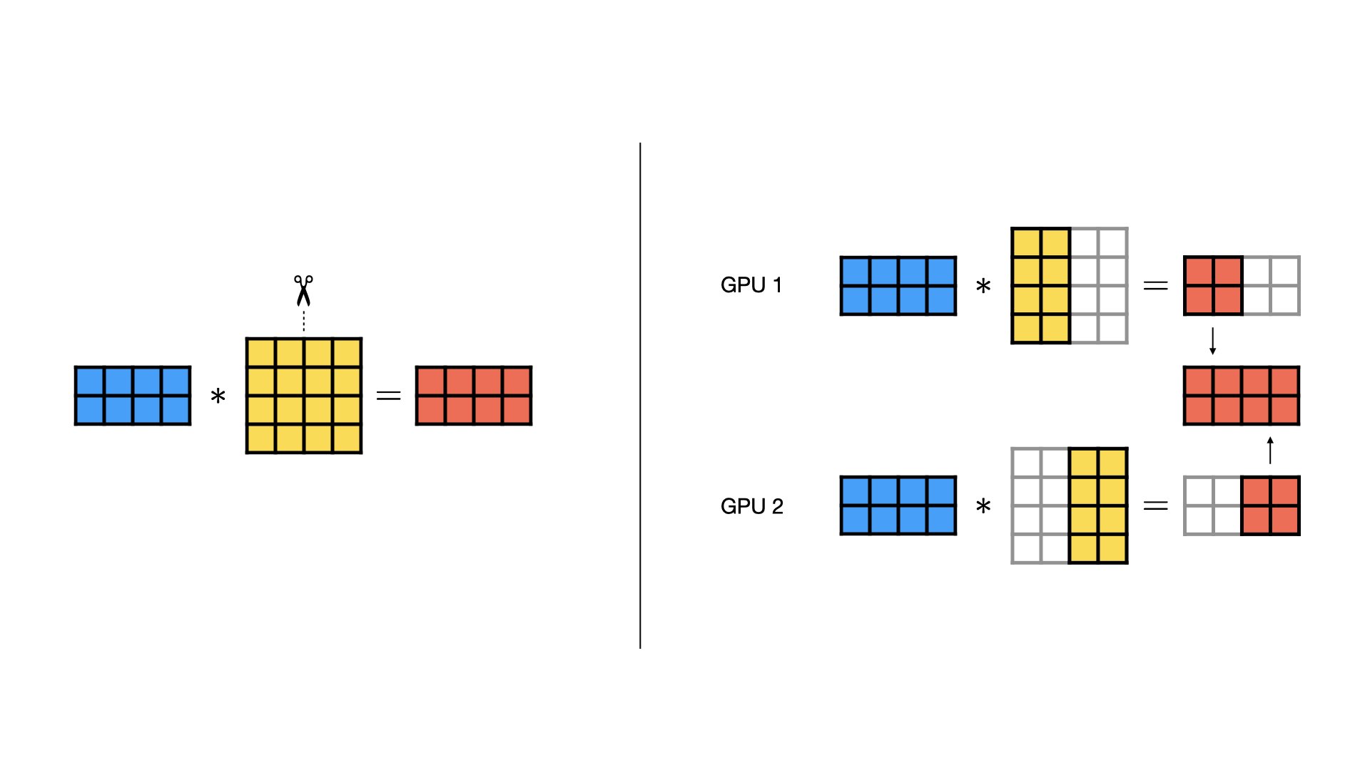
With this column-sharding setup, communication is:
- Forward pass (column sharding): each GPU produces different output features, so if the next computation needs the full activation tensor, workers exchange outputs (commonly with
all-gather). - Backward pass (column sharding): workers compute local parameter-gradient shards, then synchronize needed gradient terms (often with
all-reduceorreduce-scatter) so updates match the non-sharded model.
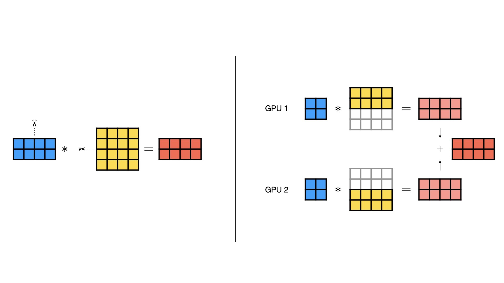
We can also shard by rows instead:
\[ W = \begin{bmatrix} W_0 \\ W_1 \end{bmatrix} \]
Now communication changes:
- Forward pass (row sharding): each GPU computes partial sums for the same output features, so partial outputs must be summed across workers (typically with
all-reduce). - Backward pass (row sharding): workers form partial contributions for shared gradient terms, so those partials are summed across workers (typically with
all-reduce) before applying updates.
As a rough sizing rule, if tensor-parallel degree is T, then each worker stores and computes roughly 1/T of a sharded layer. But communication does not shrink by the same factor, so speedup is usually sublinear. Tensor parallelism is usually combined with data parallelism to balance memory savings, throughput, and communication overhead.
5.5.5 Pipeline parallelism
In pipeline parallelism, we split the model by layers across GPUs (for example, stage 0 has early layers, stage 1 has middle layers, stage 2 has later layers). Instead of one GPU running the full network, each GPU runs only its stage and passes activations to the next stage.
For one micro-batch, the flow is:
- Forward pass: stage 0 computes and sends activations to stage 1, stage 1 computes and sends to stage 2, and so on until loss is computed.
- Backward pass: the last stage starts backprop, sends activation gradients to the previous stage, and gradients continue stage-by-stage back to stage 0.
- Each stage computes parameter gradients for its own layers, then optimizer updates are applied to that stage’s parameters.
This helps because each GPU stores only a subset of model parameters, gradients, and optimizer state. So pipeline parallelism can train deeper or larger models that would not fit on one GPU.
The main efficiency issue is pipeline bubble. At the start and end of a step, some stages can be idle while waiting for micro-batches to arrive or gradients to return.
To reduce bubbles, we usually split a batch into several micro-batches. More micro-batches improve stage utilization, but also add scheduling overhead and can increase activation-memory pressure.

Communication in pipeline parallelism is mostly point-to-point between neighboring stages (send activations forward, send activation gradients backward), rather than global collectives at every layer.
5.5.6 Interconnects and communication backends
When we scale training across multiple GPUs, communication cost often becomes the next bottleneck after math throughput. So we need to reason about link speed just as carefully as we reason about FLOPs.
An interconnect is the physical communication path between GPUs (or between servers), and its bandwidth and latency strongly affect distributed training speed.
Intra-node communication path: Within one machine, GPUs usually communicate over PCIe, NVLink, or both. PCIe is the general interconnect in most servers; NVLink is a higher-bandwidth GPU-to-GPU fabric on supported NVIDIA systems. Typical peak link rates are:
- PCIe 4.0 x16: about 256 Gbps aggregate bandwidth (about 128 Gbps each direction).
- PCIe 5.0 x16: about 512 Gbps aggregate bandwidth (about 256 Gbps each direction).
- NVLink (A100 generation): up to about 4,800 Gbps aggregate GPU-to-GPU bandwidth.
- NVLink (H100 generation): up to about 7,200 Gbps aggregate GPU-to-GPU bandwidth.
Higher-bandwidth GPU-to-GPU links reduce communication time, especially when gradients and parameter shards are large.
Inter-node network links: Between servers, training traffic goes over network fabric such as InfiniBand or Ethernet, where link speeds are on the order of 10s of Gbps in “regular” networks and 100s of Gbps in specialized HPC networks. Compared with on-board GPU interconnects, these links are usually the tighter constraint, so multi-node scaling depends heavily on minimizing communication volume and overlapping communication with compute.
Also, two clusters can have the same nominal link speed but different real performance because of topology (for example, whether all GPUs have direct high-bandwidth paths or must cross shared links). Placement can noticeably change throughput.
Communication backends: A communication backend implements collectives on available hardware. Two main contenders are NCCL and Gloo. NCCL is usually the default for GPU training because it is optimized for CUDA GPUs and high-performance collectives (all-reduce, all-gather, reduce-scatter, broadcast), and it can exploit topologies such as NVLink, PCIe, and InfiniBand. Gloo is broadly useful, especially for CPU training or environments where NCCL is unavailable, but it is usually slower for heavy GPU collective traffic.
Tuning bucket size: Most training frameworks let us tune collective bucket size. Collective bucket size is the amount of tensor data grouped together before launching one collective call (like all-reduce). Larger buckets have better bandwidth efficiency, fewer collective launches, but potentially more memory usage and less overlap of compute and communication. Smaller buckets can start communication earlier and overlap more with compute, but can add more per-call overhead.
5.6 Key terms
- activation checkpointing: A memory-saving method where we save only selected forward activations and recompute missing ones during backward pass.
- batch size: The number of training examples processed together in one forward and backward pass.
- collective: A coordinated communication operation across multiple workers, where all participants follow the same pattern.
- communication backend: The software layer that implements distributed communication primitives on available hardware.
- compute bottleneck: A limit where arithmetic throughput is the main constraint on training speed.
- data parallelism: A strategy where each worker runs the same model computation on a different shard of input data.
- distributed data parallelism (DDP): Data parallel training where each GPU keeps a full model replica and synchronizes gradients each step.
- epoch: One complete pass through the full training dataset.
- FLOPs: Floating point operations, a rough count of math work in training.
- fully sharded data parallelism (FSDP): A data-parallel strategy that shards model states across workers instead of fully replicating them.
- Gloo: A communication library often used for CPU or mixed distributed environments.
- gradient accumulation: A method where we process multiple micro-batches, sum gradients, and update parameters once.
- interconnect: A hardware link that moves data between GPUs or between servers.
- memory bottleneck: A limit where data movement or storage capacity dominates runtime.
- micro-batch: A smaller piece of a mini-batch processed as one unit inside a larger training step.
- mixed precision: A training approach that uses both reduced-precision and higher-precision arithmetic in one step.
- NCCL: NVIDIA’s communication library optimized for high-performance multi-GPU collectives.
- optimizer state: Extra per-parameter values maintained by the optimizer, such as momentum or moving averages.
- pipeline bubble: Idle time in pipeline parallelism when some stages are waiting for work.
- pipeline parallelism: Model parallelism where different layer groups are placed on different GPUs as pipeline stages.
- ring all-reduce: An all-reduce algorithm that arranges workers in a ring to spread communication load.
- task parallelism: Running different tasks concurrently, often with different control flow.
- tensor cores: Specialized GPU units for fast matrix multiply-accumulate operations.
- tensor parallelism: Model parallelism where one layer’s tensor operations are split across multiple GPUs.
Priya Goyal, Piotr Doll{'a}r, Ross B. Girshick, Pieter Noordhuis, Lukasz Wesolowski, Aapo Kyrola, Andrew Tulloch, Yangqing Jia, and Kaiming He. 2017. Accurate, Large Minibatch SGD: Training ImageNet in 1 Hour. CoRR abs/1706.02677. http://arxiv.org/abs/1706.02677.↩︎
Diego Granziol, Stefan Zohren, and Stephen Roberts. 2022. Learning Rates as a Function of Batch Size: A Random Matrix Theory Approach to Neural Network Training. Journal of Machine Learning Research 23, 173 (2022), 1-65. http://jmlr.org/papers/v23/20-1258.html.↩︎
Edward J. Hu, Yelong Shen, Phillip Wallis, Zeyuan Allen-Zhu, Yuanzhi Li, Shean Wang, Lu Wang, and Weizhu Chen. 2022. “LoRA: Low-Rank Adaptation of Large Language Models.” In ICLR 2022. arXiv version, OpenReview.↩︎
Tim Dettmers, Artidoro Pagnoni, Ari Holtzman, and Luke Zettlemoyer. 2023. “QLoRA: Efficient Finetuning of Quantized LLMs”. In NeurIPS 2023. Link.↩︎
Shen Li, Yanli Zhao, Rohan Varma, Omkar Salpekar, Pieter Noordhuis, Teng Li, Adam Paszke, Jeff Smith, Brian Vaughan, Pritam Damania, and Soumith Chintala. 2020. “PyTorch distributed: experiences on accelerating data parallel training.” Proc. VLDB Endow. 13, 12 (August 2020), 3005-3018. https://doi.org/10.14778/3415478.3415530. arXiv version.↩︎
Yanli Zhao, Andrew Gu, Rohan Varma, Liang Luo, Chien-Chin Huang, Min Xu, Less Wright, Hamid Shojanazeri, Myle Ott, Sam Shleifer, Alban Desmaison, Can Balioglu, Pritam Damania, Bernard Nguyen, Geeta Chauhan, Yuchen Hao, Ajit Mathews, and Shen Li. 2023. “PyTorch FSDP: Experiences on Scaling Fully Sharded Data Parallel.” Proc. VLDB Endow. 16, 12 (August 2023), 3848-3860. https://doi.org/10.14778/3611540.3611569. arXiv version.↩︎
Samyam Rajbhandari, Jeff Rasley, Olatunji Ruwase, and Yuxiong He. 2020. “ZeRO: memory optimizations toward training trillion parameter models.” In Proceedings of the International Conference for High Performance Computing, Networking, Storage and Analysis (SC ’20). IEEE Press, Article 20, 1-16. arXiv version.↩︎