2  Cloud computing

2.1 Preview

Before we can train models or serve predictions, we need compute that can run our code, storage that can hold our data, and networks that connect everything together. This chapter is about how that infrastructure works in cloud environments.

We will start by asking what makes something a “cloud” in the first place, then walk through the spectrum of cloud service models - from renting raw virtual machines, to bringing data to fully managed applications.

We will discuss the fundamental building blocks of cloud infrastructure: compute, networking, and storage. We will use OpenStack as a reference model because it is open source and makes the architecture explicit, and because Chameleon (which we will use throughout the course) is an OpenStack cloud.

While the first half of this unit assumes a bare-bones Infrastructure as a Service offering with bare metal or VMs as the compute instance, cloud native computing today makes heavy use of containers. So in the second half of the unit, we will introduce containers and container orchestration.

2.2 Characteristics of a cloud

When people say “the cloud” they often mean a public provider like AWS, GCP, or Azure, but you can also build a cloud on your own hardware (“on premise”). Before we get into details, let’s clarify what makes something a cloud in the first place. These “essential characteristics” of a cloud are defined by NIST.¹

On-demand self-service means you can provision resources without a human in the loop, usually via API, CLI, or web UI. If you can open a web page (or run a command line tool), launch a VM, attach a volume, and allocate a public IP without filing a ticket or waiting for someone to set up a server, you are experiencing this characteristic.

Resource pooling (multi-tenancy) means the provider runs a shared pool of physical resources and allocates slices of it to many users, using virtualization and policy to isolate them. Two research groups can share the same physical GPU servers: each group sees only its own instances, networks, and volumes, and quotas or usage limits prevent either group from capturing all of the service and starving the other group.

Elasticity (rapid scaling) means capacity can grow and shrink quickly from the consumer’s perspective. We might run a service with only one compute instance, scale to twenty during a traffic spike, and then scale back down afterward. This is enabled by the previous item; the provider has pooled resources to support many users, and their individual peak usage occurs at different times. So, one user’s idle capacity can be allocated to another user’s spike, and the provider can provision just enough total hardware to serve all users efficiently.

Network access means capabilities are available over the network using standard mechanisms. A training job might execute on a VM, write checkpoints to object storage over HTTPS, and be triggered from a GitHub Actions workflow calling the cloud API. Even when the hardware is on-prem, the interaction model is networked APIs rather than a physical console.

Metered service means usage is measured, monitored, and reported. In public clouds, this is necessary for billing. In a private cloud, the same measurements might support quota enforcement and justify future capacity expansions.

These characteristics are not always absolute. Public clouds are designed to deliver all of them strongly because their billing and scale depend on it. Private clouds (including on-prem deployments) often deliver the same interface and automation, but may be weaker on elasticity (capacity is bounded by hardware you already own, which is likely to be on a smaller scale) and on metering (you might enforce quotas rather than charge dollars per minute).

Now we understand what a cloud is: it’s a system where you can self-service provision what you need out of a shared pool of resources, scale them up or down as needed, access them over the network, and pay for what you use.

2.3 Cloud service models

What exactly are the resources provided by a cloud, though? It depends on the cloud service model.

Cloud service models are about dividing responsibility between you and a cloud service provider. As you move from the baseline (no cloud) through the cloud service models, more of the stack becomes something you consume rather than something you operate.

2.3.1 Baseline

For example, suppose I want to create a blog. Without a cloud, I would:

• purchase or find hardware
• find a place to keep it
• get power, cooling, and network access
• install an OS
• install and configure software and libraries
• … actually write the blog
• and maintain it over time, including software upgrades, physical moves, replacement parts, responding to cybersecurity incidents, and generally being the person who is called when something breaks.

This is (1) a lot of work just to keep a blog going! and (2) not at all practical for reliability or scaling.

2.3.2 Infrastructure as a Service (IaaS)

A lot of that “pain” relates to managing the hardware and physical environment. We can address some of that by renting servers in someone else’s data center: they buy the hardware, rack it, provide power and cooling, replace failed parts, and keep the physical environment running.

But a whole bare metal physical server is often more than the unit of compute users actually need. Most of the time, we want something smaller: a few CPUs and some memory for one workload. Cloud computing works at scale because of virtualization: a software layer (the hypervisor) slices one physical machine into many smaller virtual machines that we can rent on demand.

There are two common hypervisor styles:

• A type 2 hypervisor runs on top of a host OS, like a normal desktop application. This is the style we often know from laptops: VirtualBox or VMware Workstation/Fusion running a Linux VM on top of Windows or macOS. It
• A type 1 hypervisor is used in cloud infrastructure: it runs directly on the server hardware (or is integrated into the host kernel) and exists primarily to host VMs efficiently. KVM is one example of this type of hypervisor.

This type of service - bare metal servers or VMs on demand - is the most fundamental cloud service, and is known as IaaS, or Infrastructure as a Service. Instead of buying hardware, plugging it in, and managing all of that, we go to a cloud service and say: “I would like one virtual machine with two CPUs and an Ubuntu 24 operating system, please.” Once we launch our compute instance, we have full control over what runs inside it.

In this service model, the cloud service provider is responsible for the physical hardware and the hypervisor (the layer that creates VMs and allocates hardware resources to them). Everything above that (the OS, libraries, application code, and application data inside your VM) is your responsibility. In my blog example, I wouldn’t have to buy the server, find physical space for it, or plug it in, but I’d still have a lot more to do than just writing blog posts.

2.3.3 Container as a Service (CaaS)

What if I wanted to offload some of this work - say, managing the OS and OS updates? We can take virtualization another step beyond VMs, and virtualize access to the operating system. In a container environment, the hardware and host operating system live outside the container, and a container engine manages access to the host OS and isolation between containers (analogous to how a hypervisor manages access to hardware for VMs).

When the unit of compute is a container, rather than a VM, the user no longer has to manage or maintain an OS. But, the user is still responsible for bringing their own container “blueprint”, which sets up their application runtime; and their own application code. For example, to run a simple Flask web site in a container, I might use the following to describe the environment I want in my container -

FROM python:3.11-slim

WORKDIR /app

COPY requirements.txt .
RUN pip install --no-cache-dir -r requirements.txt

COPY app.py .

EXPOSE 5000

CMD ["python", "app.py"]

which says “base it on Python 3, install these libraries, copy in my app code, and run app.py on start”. The cloud service provider will build that container for me, and then run it. Here’s what app.py might look like in this case:

from flask import Flask
app = Flask(__name__)

@app.route("/")
def hello():
    return "Hello from Flask"

if __name__ == "__main__":
    app.run(host="0.0.0.0", port=5000)

In my blog example, I might use a pre-defined container “blueprint” for an open source blogging platform, like Wordpress or Ghost. I would still be responsible for setting up plugins, migrating to a new updated container “blueprint” when there is a Wordpress or Ghost update, and of course, writing my blog posts - but without having to manage an OS, and especially with being able to use “known good” container blueprints, I’ve saved myself a lot of work.

This type of offering is known as CaaS, or Container as a Service.

Beyond the basic role of “running containers”, the cloud service provider often offers services where they will manage container orchestration, which we’ll discuss further in a later section. But we note at this point that a major benefit of this type of service is that with container orchestration, the cloud provider can take over responsiblity of scaling my service in response to demand. Under heavy load, it will scale up (and my costs will scale up accordingly); under low load it will scale down (and my costs will go down).

2.3.4 Platform as a Service (PaaS)

Can I offload even more responsiblity? Of course! Suppose the Flask environment described in the previous section is a very popular, standard environment, and many users are building application code on top of it. Instead of making me bring my own “blueprint”, with the responsibility of selecting and updating Python versions, library versions, etc. the cloud service provider can give me a known application runtime and says: “Give me your application code, and I will run it for you in this environment.”

I just bring app.py which defines the application code:

from flask import Flask
app = Flask(__name__)

@app.route("/")
def hello():
    return "Hello from Flask"

if __name__ == "__main__":
    app.run(host="0.0.0.0", port=5000)

and the cloud service provider handles everything below it. This type of offering is known as PaaS, or Platform as a Service.

2.3.5 FaaS

In the example above, notice that my application mostly exists just to run a function and make it available at some endpoint on the Internet. The hello() function returns “Hello from Flask” when I visit the URL http://A.B.C.D:5000/ (the address A.B.C.D come from the cloud service provider, the 0.0.0.0 in the code is not a real address but just means “listen on every address that I have”).

When I just need to run a function in a known environment and application context, I can use a FaaS offering, Functoin as a Service, often called “serverless”. This shifts responsiblity again - I bring

def handler(event, context):
    return {
        "statusCode": 200,
        "body": "Hello from function"
    }

without needing complete application code. The cloud service provider takes care of deploying it to an Internet endpoint within a known environment and application context. The cloud service provider can also scale it according to load, and I will likely pay only when the endpoint is used, instead of having to pay for an always-on compute instance in case it is needed.

2.3.6 Software as a Service (SaaS)

Sometimes, a user just needs to bring data - like in my blog example, where I want to write blog posts but do not want to manage hardware, OS, software stacks, or custom functions. For popular software, the cloud service provider can make this a reality by offering a SaaS, or Software as a Service, offering.

With SaaS, the provider operates the infrastructure and the application, and the user’s role is limited to configuration and content. In the blog example, this would be a managed Wordpress or Ghost service: they run everything, and all we have to do is write blog posts and bring our own content.

2.3.7 Overview

At one extreme (IaaS), the provider brings basic infrastructure, and we build everything on top of it. At the other extreme (SaaS), the provider manages everything and we just bring our own data. Here’s a summary of the cloud service models we introduced:

As we move along the service-model spectrum, we are also moving toward managed services: the provider takes over more of the work of operating pieces of the stack. Modern commercial clouds (AWS, GCP, Azure) all provide IaaS, and many also provide container services, serverless functions (FaaS), and potentially SaaS products. But beyond the core compute models, cloud providers also often offer managed databases, data warehouses, storage, and also higher-level ML offerings like managed training/inference platforms. Some providers specialize and only offer one piece (for example, a backend-as-a-service like Supabase, or frontend hosting plus serverless functions like Vercel).

In this course, we will mostly work with IaaS (using Chameleon) and build everything else on top of raw infrastructure. We do that, first, because we want the experience of building our own services on top of base infrastructure so we can see what managed services are abstracting away. Second, it is more transferable: if we only learn one specific managed product, we can end up with skills that are specific to that product. If we learn how to bring up and operate a service ourselves, we can generalize those ideas across clouds and across managed service offerings. Later in the course, when we talk about commercial clouds, we will also look at some managed services directly.

This shift toward managed services also comes with a shift in mindset about how we operate compute. In the traditional “pets” style, we treat servers as special: we name them, patch them in place, remember their quirks, and try to avoid replacing them (because it’s a lot of work to do!). In the cloud-style “cattle” approach, we assume machines and containers will come and go: we recreate them from an image or template, replace them when something goes wrong, and keep important state in durable services (databases, storage) that outlive any compute instance. Managed services make this easier because more of the stack is already designed to be automated and replaceable. We will follow up on this idea in a future unit.

2.4 IaaS building blocks

Cloud service models divide responsibility between you and a provider, but they all build on the same underlying primitives: compute (where code runs), network (how traffic flows), and storage (where data persists).

2.4.1 Compute

In IaaS, the core compute product is a compute instance or server. This is the temporary, provider-managed “slice” of compute that we lease. An instance has an identity (ID or name), a lifecycle (boot, reboot, stop, start, terminate), allocated resources (CPU, memory, and optionally GPU), and attached storage and network interfaces.

Most IaaS instances are virtual machines (VMs) running on a hypervisor. Some providers also offer bare-metal instances which can be useful for performance isolation or for specialized hardware access.

Commercial clouds use different product names for the basic VM service:

Service	GCP	AWS	Azure
VM instance	Compute Engine	EC2	Azure Virtual Machines

When you “launch” an instance in IaaS, you are going to be asked to specify a launch configuration, including:

• the instance type or flavor (CPU, memory, and optionally GPU, from a list of “types” curated by the provider)
• provisioning type (on-demand, reserved/committed, or spot/preemptible)
• the image (what template of an OS + base software to boot, from a list of images available from the provider)
• storage (root disk and any additional volumes)
• networking (which networks/subnets, private/public IPs)
• firewall rules (which inbound/outbound traffic is allowed)
• identity and permissions (what cloud services on your account the compute instance can access)
• access (SSH keys)

For example, this is the interface for launching a VM instance on GCP’s Compute Engine service:

Start from the cloud console and click Create a VM in the right project.

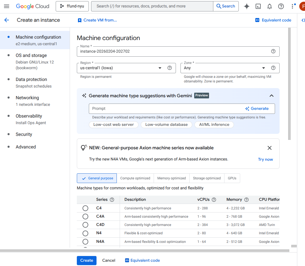
Choose placement: set the instance name, region, and zone.

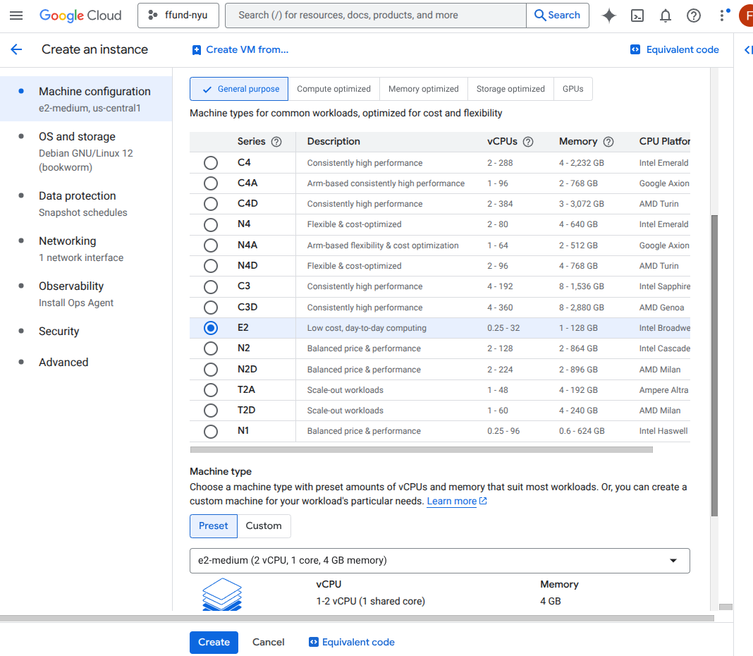
Choose machine type (CPU and memory): for example, an e2-medium with 2 vCPU and 4 GB RAM.

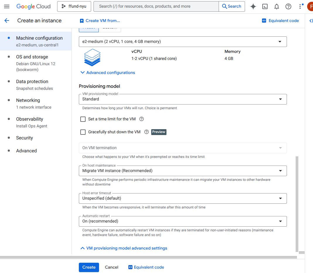
Choose the provisioning model (on-demand vs spot/preemptible) and lifecycle behavior.

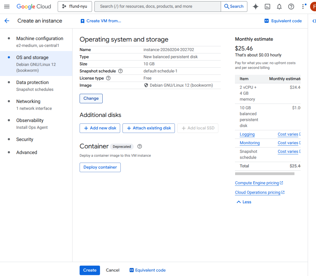
Choose the boot image and disk settings (OS and boot disk type/size), and optionally attach additional disks.

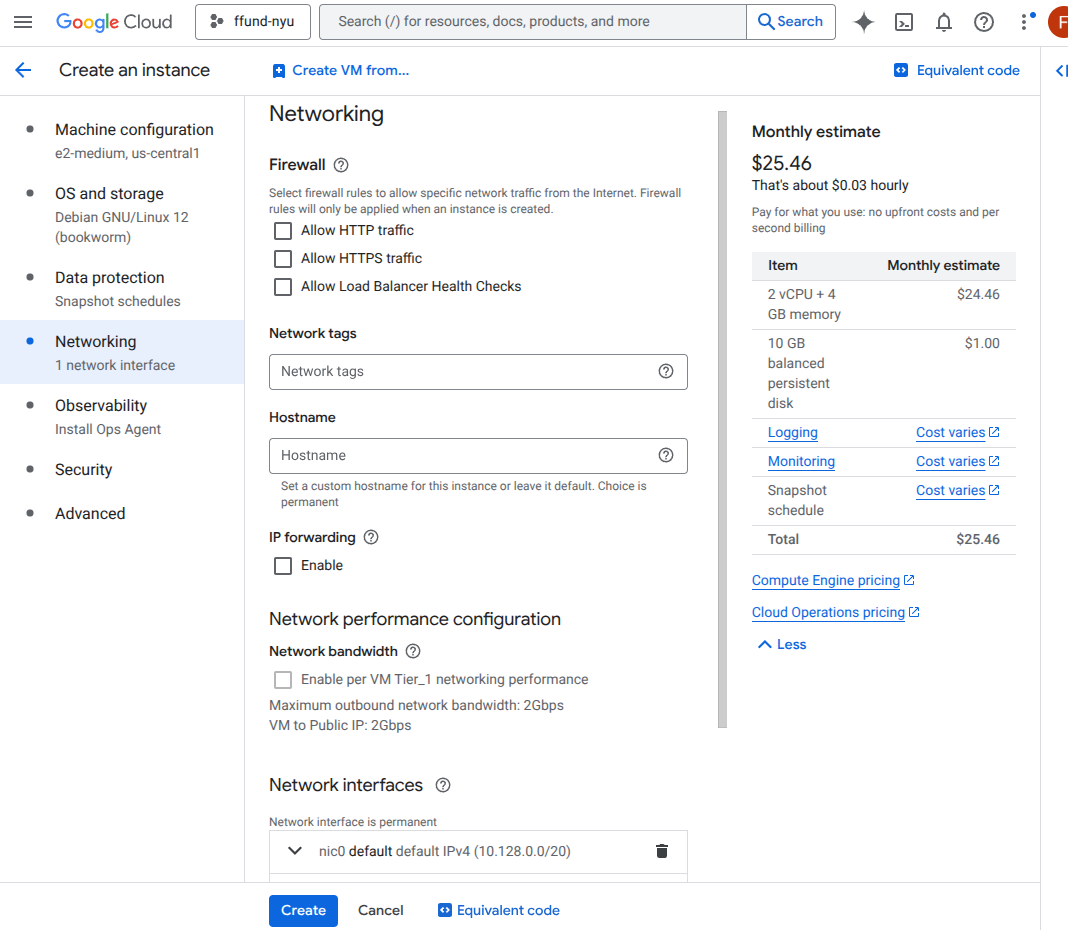
Configure networking and firewall rules: network/subnet, public IP, and allowed inbound traffic (like HTTP/HTTPS).

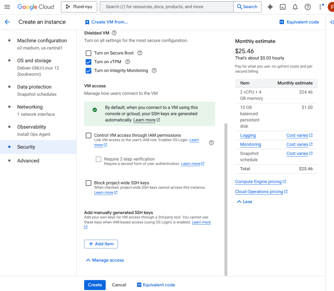
Configure access and security controls.

And here is the same process on AWS:

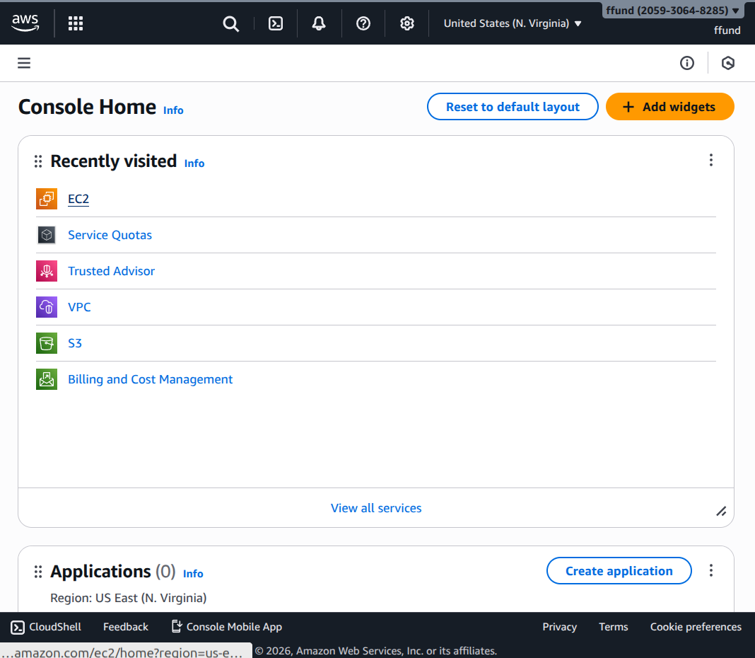
Open EC2 in the AWS console.

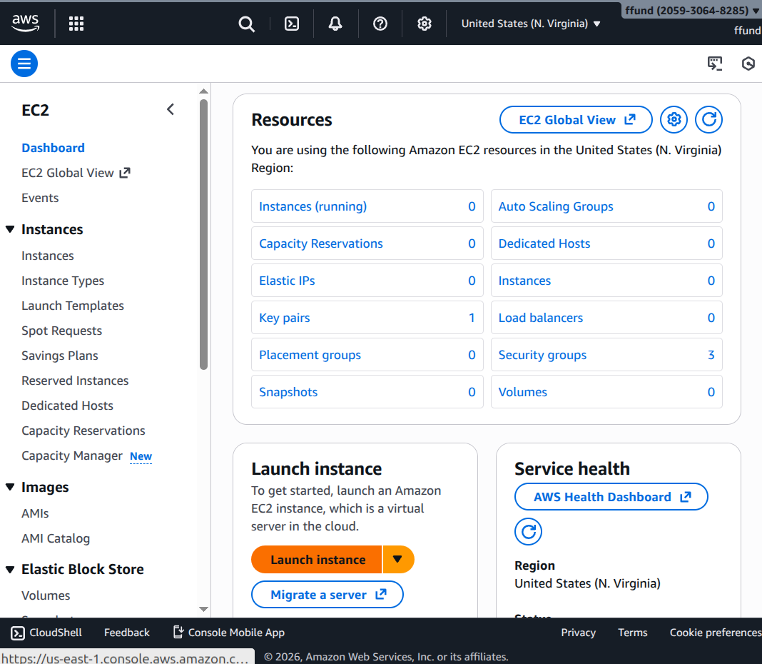
Start the instance launch wizard.

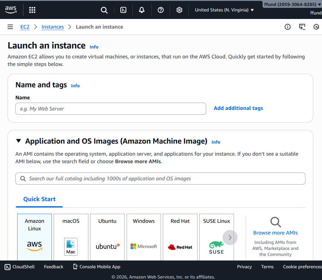
Set the instance name.

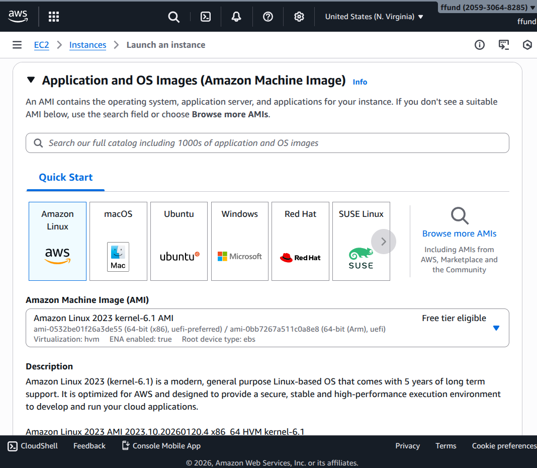
Choose the image to boot.

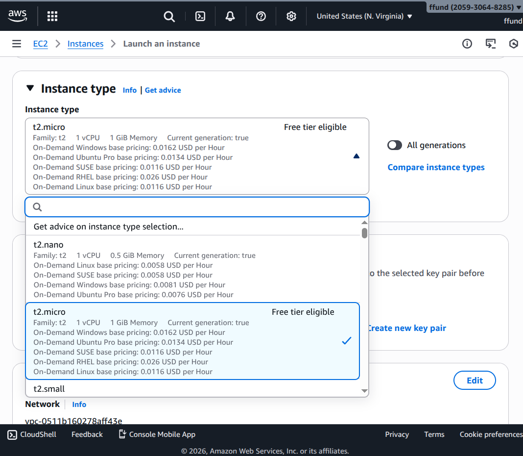
Choose the instance type (CPU and memory).

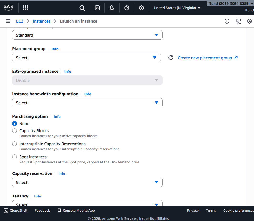
Choose provisioning type (on-demand vs spot).

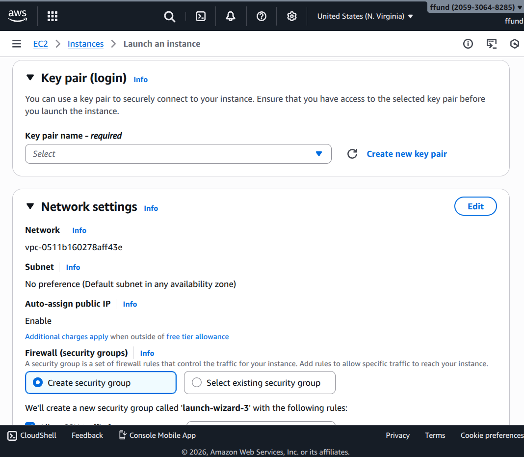
Choose access (SSH key pair).

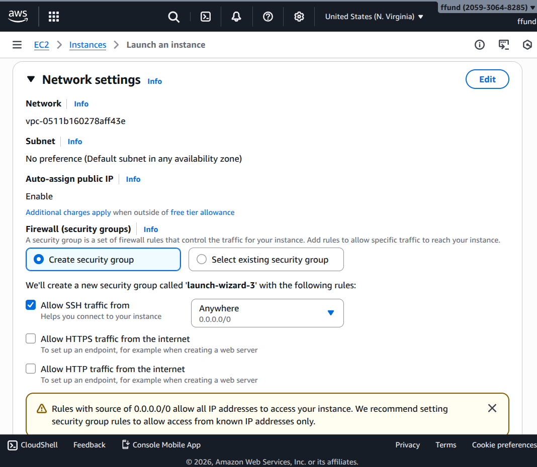
Configure networking and firewall rules.

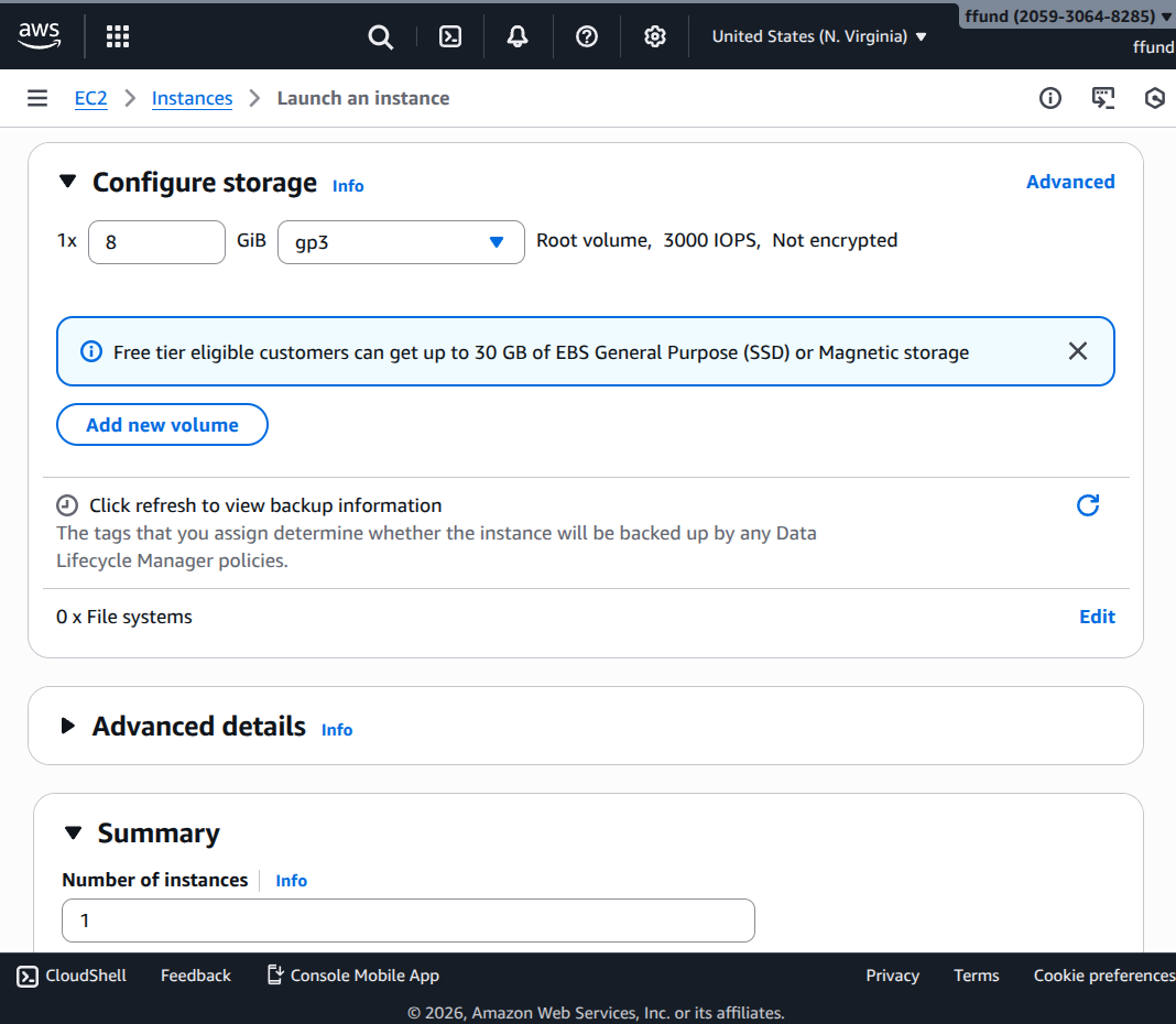
Configure storage.

The idea is similar on an OpenStack cloud like Chameleon. Chameleon only offers compute by reservation, not on demand, so we start by creating a lease for some compute:

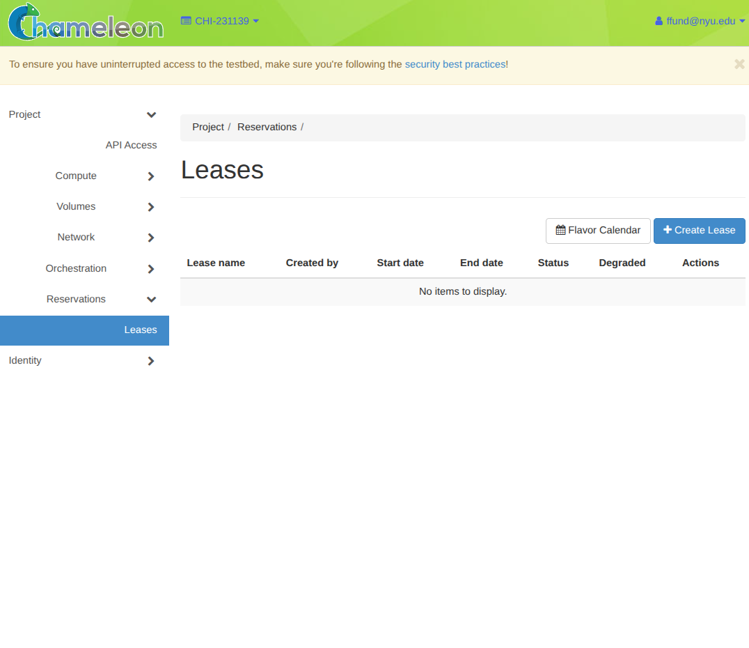
Open Reservations -> Leases, then click Create Lease.

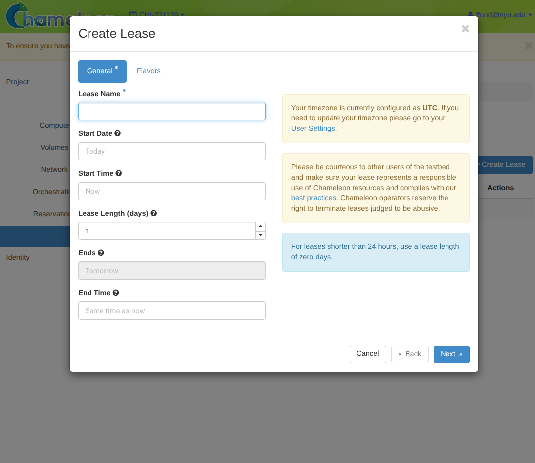
Choose the lease name and time window (start and length).

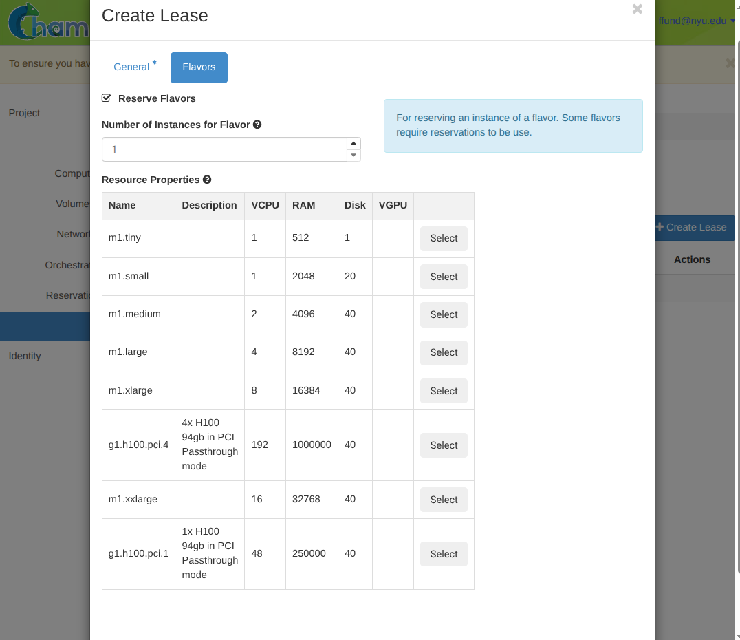
Choose the instance type(s) (flavors) and how many to reserve.

and then we can launch an instance using that lease:

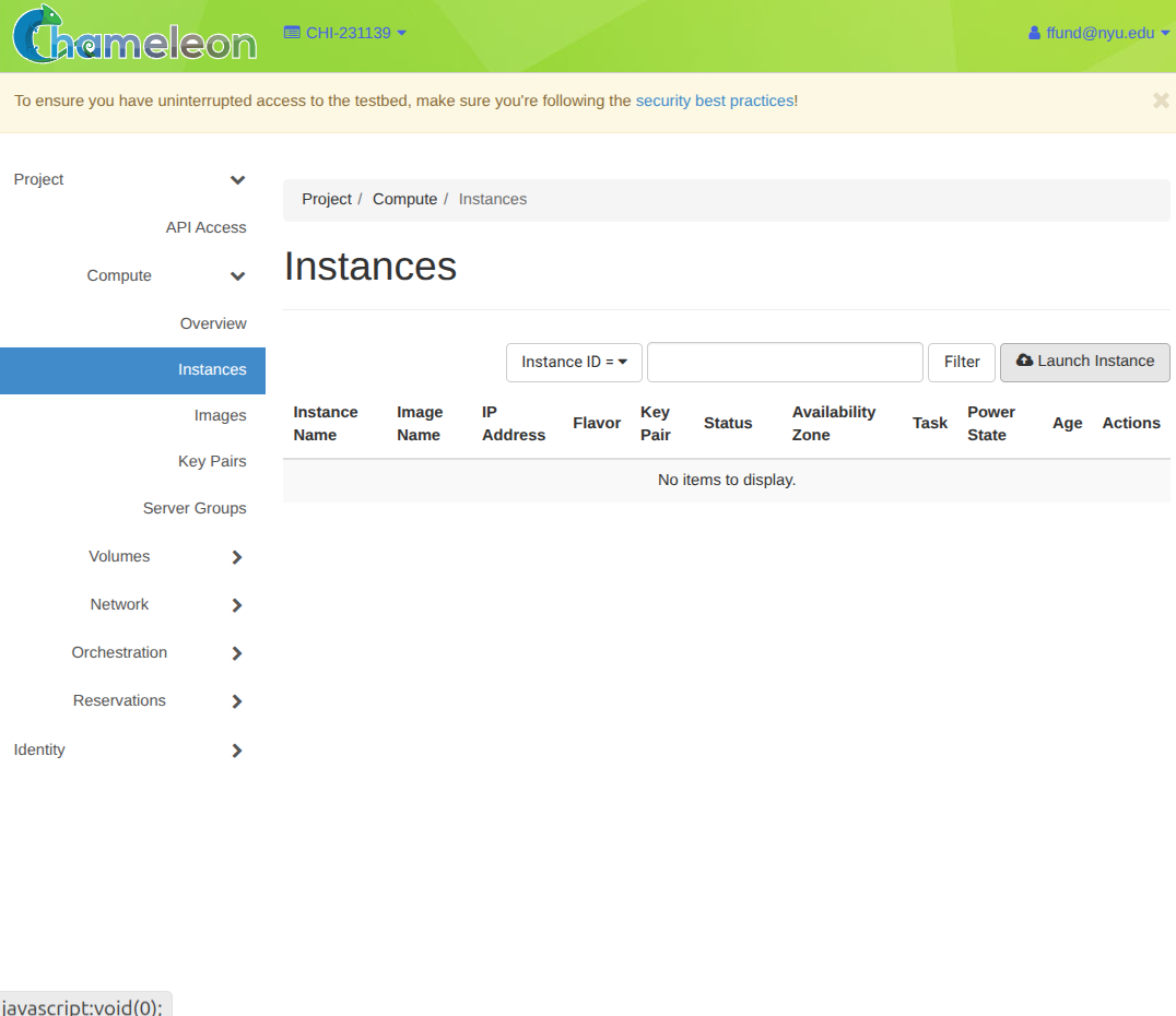
Start the launch wizard (Compute -> Instances -> Launch Instance).

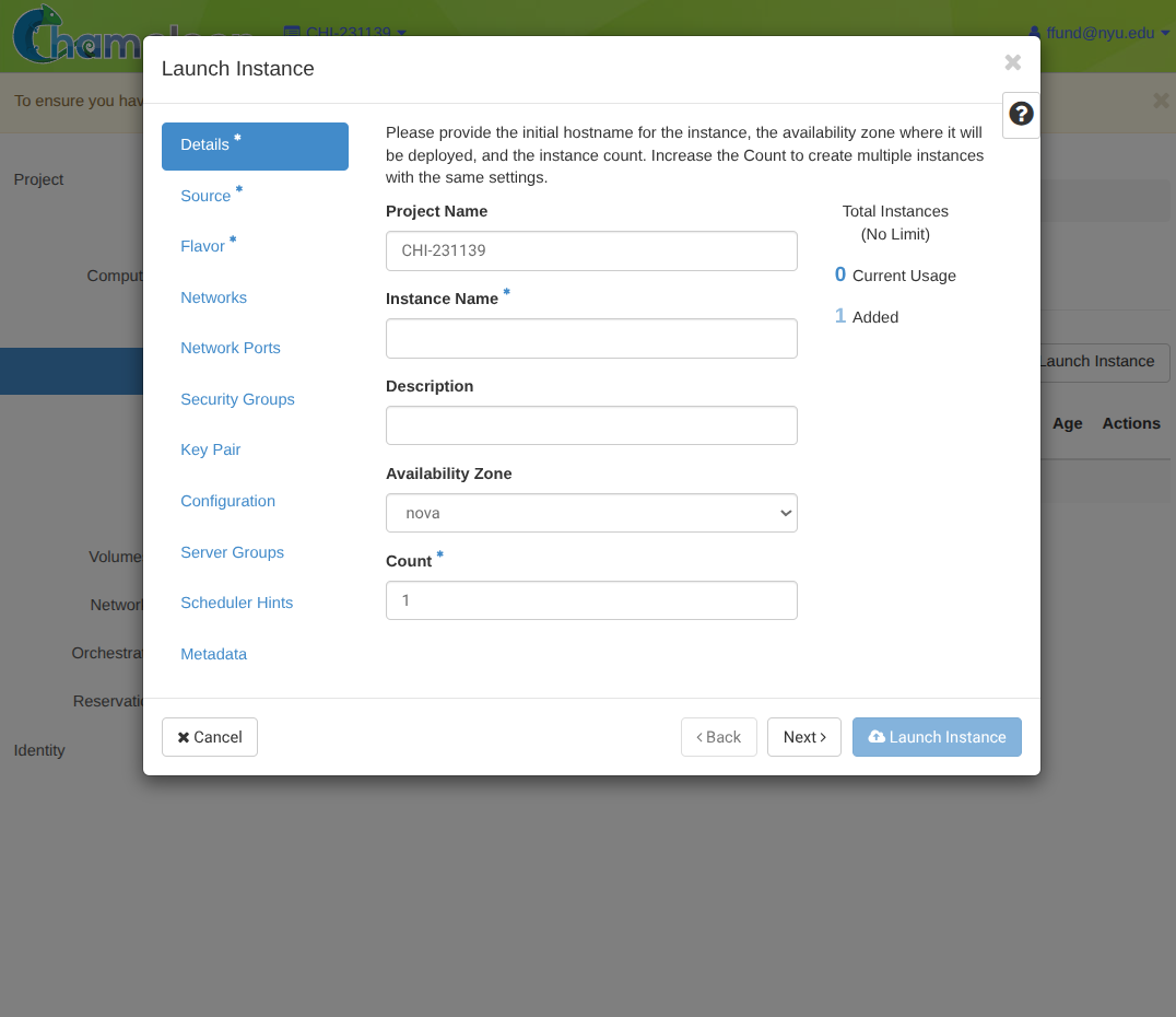
Set basic instance details, such as name.

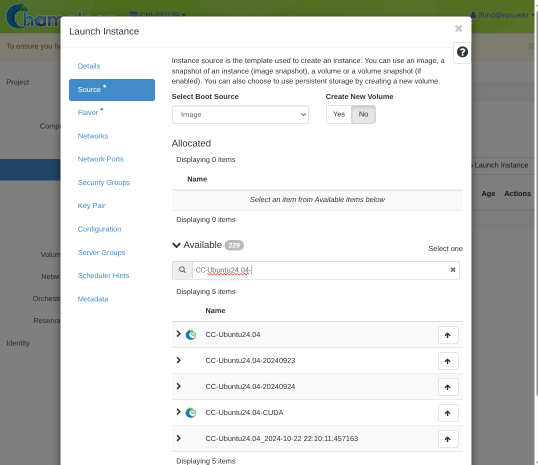
Choose the image to boot.

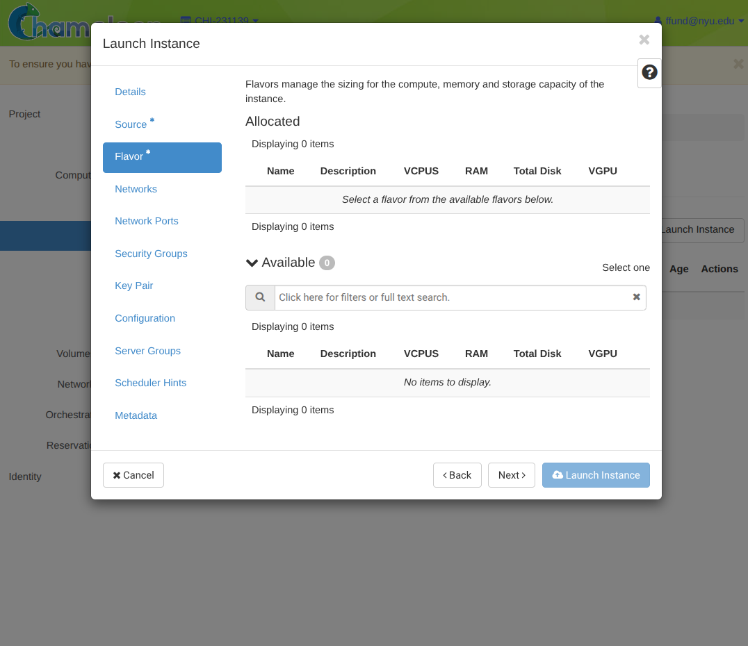
Choose the instance type, or flavor (from among active leases).

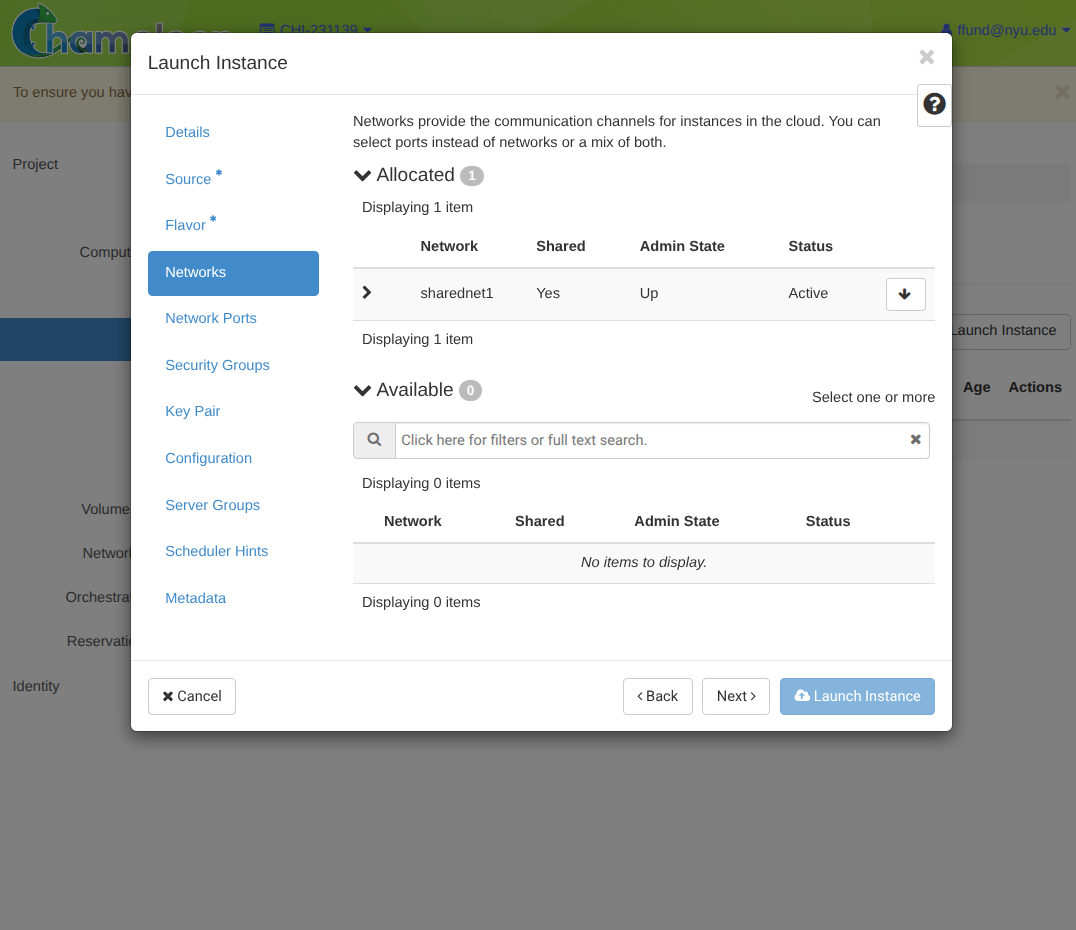
Configure networking (select network to attach to).

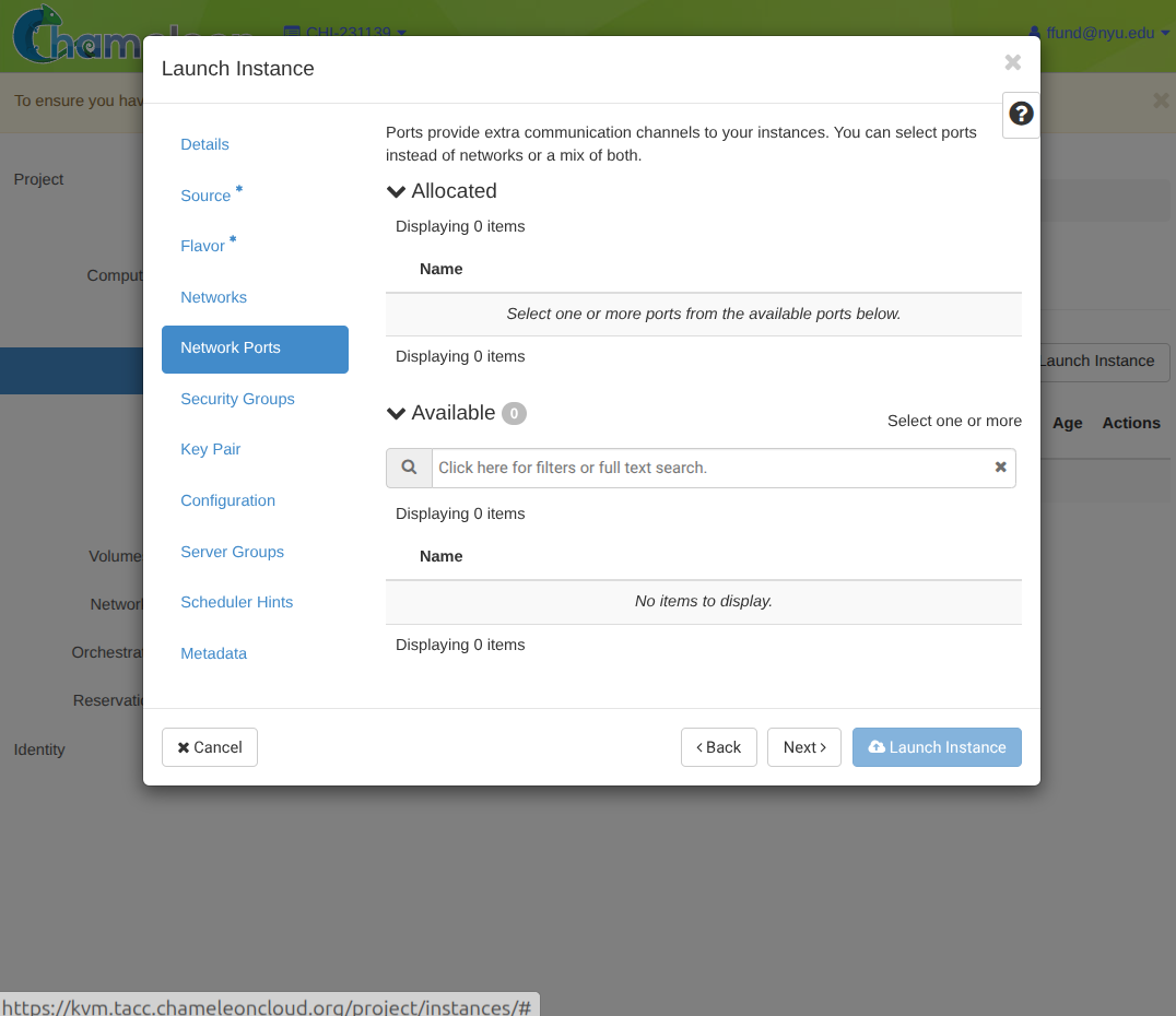
Select network ports to attach.

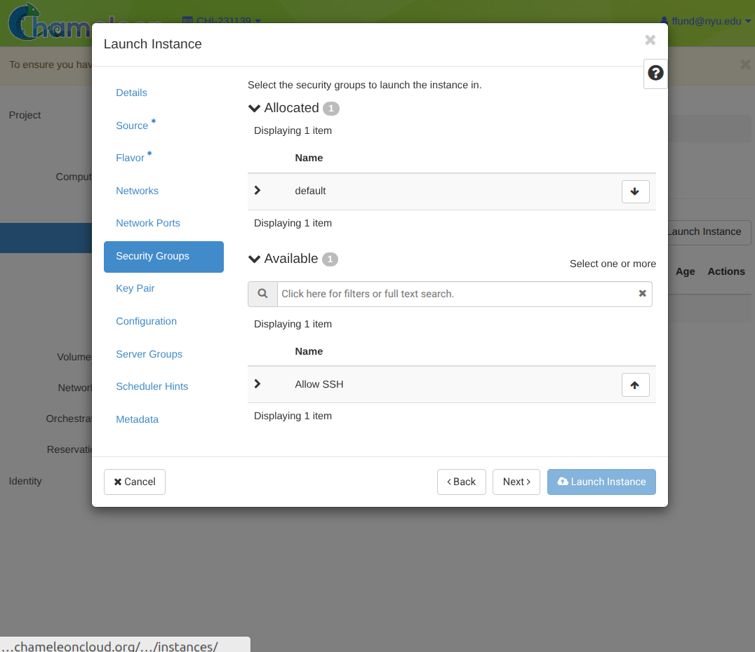
Configure firewall rules (security groups).

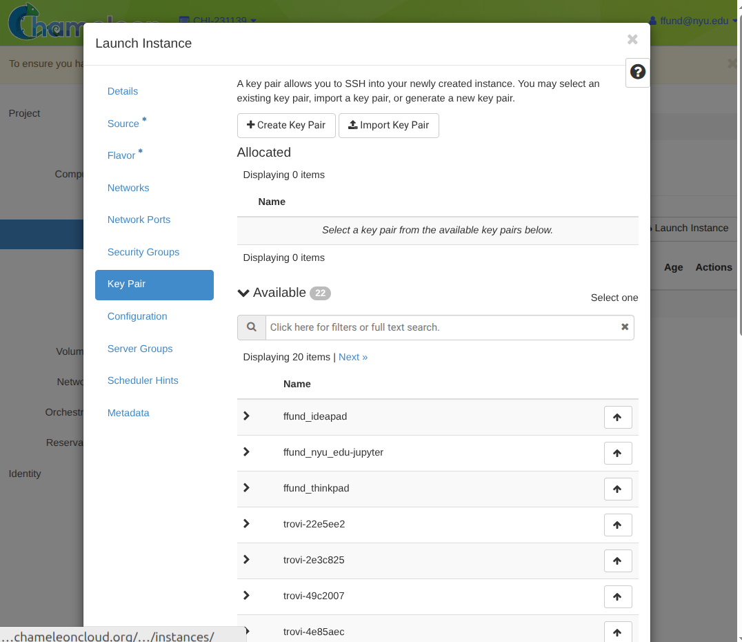
Configure access (SSH key pair).

The interface may look different across clouds, and some clouds have options that are not available on other clouds, but once you are familiar with cloud compute you can see how the ideas translate from one cloud to another.

2.4.2 Network

Before getting into cloud-specific networking, it helps to understand how network communication works at a fundamental level.

The TCP/IP protocol stack organizes networking into layers, each with its own responsibility and its own identifiers. This layered model is the foundation for everything else. For our purposes, we are mostly concerned with the identifiers used at each layer, which are used to answer the fundamental question of “Is this received packet for me?”

• Physical layer: transmits bits as electrical signals, light pulses, or radio waves over a physical medium. This is invisible to use in the cloud context, except in the sense of “if there is something wrong with the physical link then the network is down”.
• Link layer (also called data link or network access): transfers data between devices on the same network, e.g. between devices plugged in to the same switch. This requires local addressing (MAC addresses), so that we can specify the source and destination of any link layer frame on a network. Link layer addresses look like six pairs of hex digits, separated by : characters, like: 00:22:44:66:aa:cc.
• Network layer (also called Internet layer): transfers data across different networks. This requires global addressing (IP addresses), so we can specify the original source and final destination of any network layer packet. The global address is not necessarily the same as the local address, as packets are forwarded from one network to the next; while the global destination is the network layer address of the final destination, the local address is the link layer address of the next router within the network who will forward the packet on toward its destination. IPv4 addresses look like four decimal digits in the range 0-255, separated by ., like: 12.34.56.78.
• Transport layer: provides end-to-end communication between processes. There are two transport layer protocols - TCP and UDP - and they each use integer port numbers as identifiers. Some types of processes have well-known port numbers, like HTTP (TCP port 80), HTTPS (TCP port 443), and SSH (TCP port 22); other processes use ephemeral port numbers, which means they randomly select from a range of large numbers until they find one that is not used. When a host receives a packet whose destination at the transport layer is “TCP port 45183” it will check which process is using that port, then place the packet in the receive buffer for that process.
• Application layer: this is where the data that will be sent over the network comes from! Applications use the socket API to interact with the network. This API allows the application to say things like “Listen for incomming connections on port X”, “give me the packets waiting in the receive buffer for port Y”, “send a packet to destination Z”, and so on.

Let’s look at these layers from the point of view of a single host (e.g. a VM or a bare metal server). A host can have one or more network interface cards (NICs). Each NIC handles the physical layer (bits on a wire or radio waves) and participates in the link layer (how to send traffic to another device on the same physical medium). Above that, the operating system takes responsiblity for the network layer and the transport layer.

Where each layer of the TCP/IP protocol stack “lives” on a host: applications in user space, transport and network layers in the kernel, and link/physical layers partly in the kernel and partly in the network interface card (NIC) hardware/firmware.

Now, let’s look at how communication happens across networks.

Networking across networks.

In this figure, the host on the left (IP 1.1.1.1) initiates an SSH connection to the host on the right (IP 4.4.4.4). SSH is a TCP service that listens on port 22, so the SSH client opens a TCP connection from an ephemeral client port (here 56789) to the server’s SSH port: 1.1.1.1:56789 -> 4.4.4.4:22.

The IP header stays end-to-end: source IP 1.1.1.1, destination IP 4.4.4.4. But the link-layer (MAC) addresses are only local to one physical network, and 4.4.4.4 is not on the sender’s local network. First, the sender checks its internal routing table to find out what router will forward packets to that destination, and via which of its NICs. It will then put the router’s MAC address, ending in :cc, as the destination address of the frame, and transmits it on network 2. The switch shown inline forwards frames transparently to the router.

The router then strips the old link-layer header, consults its routing table, and forwards the same IP packet out of another NIC onto network 3, creating a new link-layer frame with new source and destination MAC addresses (ending in :dd and :ee respectively).

Finally the destination host receives a frame whose link-layer destination is its own MAC, sees that the IP destination is 4.4.4.4, and delivers the payload to the process listening on TCP port 22 (the SSH server).

So far, all of the IP addresses we used were assumed to be globally routable. In fact, there are public IP addresses and private IP addresses.

• Private IPs can be reused in many separate networks, but they cannot be reached directly from the internet. The private IPv4 ranges are 10.0.0.0-10.255.255.255, 172.16.0.0-172.31.255.255, and 192.168.0.0-192.168.255.255.
• Public IPs can be reached from the internet, but they must be globally unique across the entire Internet! So, they are scarce and are usually allocated more carefully (often one public IP for an entire service, not one per instance).

Given this distinction between private and public addresses, let’s reconsider the example from earlier, but now the host on the left has a private IP address. This figure shows a common pattern in networking: source NAT (SNAT) for outbound access. The host starts with a private IP (for example, 192.168.10.49) and initiates an SSH connection to a public destination (for example, 128.238.38.77:22) from an ephemeral port (56789). When the packet reaches the router/NAT gateway, the gateway rewrites the source IP from the private address to a public address it owns (for example, 24.186.213.20) and records a mapping like 24.186.213.20:56789 <-> 192.168.10.49:56789. Replies from the internet come back to 24.186.213.20:56789, and the gateway uses that mapping to translate them back to the private IP and forward them to the original host. This is how instances with only a private address can reach the internet without being directly reachable from it.

Networking across networks with source NAT.

We can take a similar approach in the opposite direction. Our instances have private IPs that the internet cannot route to. So how can an outside client reach a service running on a private instance? DNAT is what makes “public IP -> private IP” (or “public IP:port -> private IP:port”) work. When we set up an instance in the cloud, it is assigned a private IP address. However, we can also associate a floating IP or elastic IP address, which is a public IP address allocated to us by the cloud provider, with that same network interface. Then, when a packet arrives from the internet addressed to the public IP (and perhaps a specific port, like TCP 22 for SSH or TCP 443 for HTTPS), the cloud edge device rewrites the destination to the instance’s private IP (and port) and forwards it inside the cloud network.

To receive traffic from the Internet, we also need to configure security groups: a set of rules that says what traffic is allowed to reach an instance and what traffic it is allowed to send. Most clouds are “default deny” for inbound traffic: even if we have a public IP and DNAT is set up, nothing can connect unless the security group allows it. For example, to SSH into an instance we will allow inbound TCP port 22 (often only from our own IP range). To run a web service we will allow inbound TCP ports 80 and/or 443. Everything stays blocked unless we explicitly open it.

SNAT and DNAT explain how private instances reach the internet and how the internet can reach private instances through a public endpoint. Now we will zoom out and name the cloud object that ties these pieces together: the VPC. In the cloud, networking is virtualized, just like compute, and the typical unit of “network” that we work with in the cloud is a VPC. It’s not a physical Ethernet segment - it is a set of networking objects and rules that makes it look like we have our own private network.

• When we “create a network” in a cloud, it usually means: define a virtual network segment and choose an address range (a “subnet”) that will be used for private IPs on that network. The cloud will then allocate private IP addresses from that range as we attach instances to it, or we can allocate them ourselves.
• When we “create a port”, it means: we create a virtual NIC attachment point on a particular network. That port gets a MAC address and one or more private IP addresses, and we can attach it to an instance. In other words, a port is the concrete thing that puts a VM onto a network.
• When we should “create a router”, it means: create a virtual router that can forward traffic between networks. If we attach the router to an “external” network, it also becomes the boundary to the Internet.

From our perspective, we are wiring networks together. But under the hood, the cloud is installing and updating forwarding rules in a switch so traffic goes where we intend.

What it looks like: virtual networks and a router.

What it really is: forwarding rules on a switch.

Given these building blocks of networks in the cloud, some typical patterns you will see include:

• Bastion (jump host): we keep most instances on private IPs and do not give them public endpoints. Instead, we SSH into one instance that has a public IP, and then SSH from that instance to the private instances. Security groups are configured to allow inbound SSH to the bastion, and to allow inbound SSH to private instances from the bastion.
• Private cluster with a head node: sometimes we want many private instances to exchange data with one another freely (for example, distributed training workers that need to communicate and share artifacts), but we still want one “head” node that we can reach from the internet. One way to do this is to give the head node two network ports: one on a public-facing network (with a public IP via DNAT) and one on the private cluster network. The worker nodes have private ports on the private network; they may also have a port on the public network for outgoing connectivity via SNAT, but no public IPs on these ports. Inside the private network, security groups can be relatively open so workers can talk to each other.
• Three-tier networks: we create a public-facing network that holds the frontend with a public IP (via DNAT). Then we create a private network for frontend-to-app traffic, and another private network for app-to-data traffic. The frontend instances have one port on the public network and one port on the app network; the app instances have one port on the app network and one port on the data network; and database instance have only a port on the data network.

2.4.3 Storage

The third fundamental ingredient of an IaaS offering is storage.

There are two major storage primitives: block storage and object storage. You are already familiar with block storage: your laptop hard drive, USB thumb drives, etc. are examples of block storage. Object storage works very differently: it is accessed over a network using APIs. We will discuss object storage in more detail when we get into data systems, but here we focus on block storage and how it directly relates to compute instances.

The fundamental unit of block storage is a volume. There are different types of volumes:

Root disk (bootable volume) vs data volumes. Every instance has a root disk (the disk that contains the OS and that the machine boots from). Many systems also attach additional volumes for data. A boot volume is a root disk that is bootable, while a data volume is an extra disk that is not used to boot. Inside the instance, a volume appears as a block device (for example /dev/vdb). You typically create a filesystem (ext4, xfs, etc.), and mount it at a path (for example /var/lib/postgresql/data).

A bootable volume is often created from an image as a starting point, i.e. be backed by an image. An image is essentially a disk snapshot plus metadata.

Ephemeral vs persistent volumes. A persistent volume outlives the instance; when the instance is terminated, the volume still exists (and we still pay for it!) and can be attached to another instance in the future, with data stored on it still intact. Ephemeral storage is deleted when your instance is terminated, so all data on it is lost.

2.4.4 OpenStack as a reference

We use OpenStack here as a reference model because Chameleon Cloud runs an OpenStack software stack. OpenStack is an open source framework for running your own cloud, including an on-premise cloud.

OpenStack is not one program. It is a collection of services; each user-facing idea (“compute”, “network”, “storage”) is implemented by one or more OpenStack services. The framework also includes shared services, such as authentication, and user interfaces.

Function	OpenStack service(s)	What it provides
Compute	nova	VMs: create, delete, reboot, resize, schedule
Compute	ironic	Bare-metal provisioning as “instances”
Compute	zun	Containers in OpenStack (less common; many deployments use Kubernetes via Magnum instead)
Networking	neutron	Virtual networks, subnets, routers, ports, security groups
Networking	octavia	Load balancing
Storage	cinder	Block volumes
Storage	swift	Object storage
Storage	manila	Managed file shares
Shared services	keystone	Identity, projects/tenants, roles, tokens
Shared services	glance	VM images
Interfaces	horizon	Web UI
Interfaces	openstack CLI	CLI (often via python-openstackclient) and SDKs

Commercial clouds are built on similar services, but with other names; and their implementations are not open source. On an OpenStack cloud, we can peek under the hood and see how all the pieces fit together.

2.5 Containers

So far, we have assumed that the basic unit of compute is a VM or a bare metal server. But in practice, we will work mostly with containers - whether by deploying a container on a CaaS offering, or by running our own container engine inside an IaaS VM, and using that to run containers.

When people first deploy software on cloud compute instances, they often treat the instance like a long-lived server: install packages, modify configs, SSH in to debug, and apply hotfixes whenever a problem occurs. That approach works at small scale, but it breaks down quickly. Different services want different system libraries, configurations drift over time, and it becomes extremely painful to replace an instance. One response is a container. Instead of treating the machine as the unit of deployment, we treat a packaged application environment as the unit of deployment. If we need to change that application environment, we do not make changes directly on running instances; we change the package and then deploy a new instance of the package.

2.5.1 Building an image

A container image is the artifact you build and ship. A container image is built from a “blueprint”, most commonly a Dockerfile. At a high level, an image contains a filesystem snapshot (your application plus dependencies) and metadata such as default command/entrypoint, environment variables, working directory, and optional exposed network ports.

Here is a small, realistic example for a Python service:

FROM python:3.12-slim

WORKDIR /app

# Install deps first so Docker can cache them.
COPY requirements.txt /app/
RUN pip install --no-cache-dir -r requirements.txt

# Copy the application code.
COPY . /app/

# Run as a non-root user.
RUN useradd -m appuser && chown -R appuser:appuser /app
USER appuser

EXPOSE 8000
CMD ["python", "-m", "uvicorn", "server:app", "--host", "0.0.0.0", "--port", "8000"]

The core Dockerfile instructions map to common build steps. FROM chooses a base image (e.g. an image for your preferred runtime). RUN executes commands at build time to install dependencies. COPY and ADD bring application code and other assets (configs, scripts, static files) into the image. ENTRYPOINT and CMD define what runs when the container starts. You may also encounter USER (run the next instructions as a different user), ENV (set environment variables), WORKDIR (change working directory in which to run the next instructions), EXPOSE (document which network ports the containerized service expects to listen on), and ARG (build-time variables).

Here is a second example that you might use to set up a common environment for ML training within an organization: it will build a Jupyter + PyTorch + CUDA base image, plus a team’s Python dependencies, plus a few environment variables that configure where artifacts will be written.

FROM quay.io/jupyter/pytorch-notebook:cuda12-python-3.12

WORKDIR /home/jovyan/work

# Install Python deps in a cache-friendly way.
COPY requirements.txt /tmp/requirements.txt
RUN pip install --no-cache-dir -r /tmp/requirements.txt

# Configuration for artifact storage 
ENV AWS_REGION=us-east-1
ENV S3_BUCKET=my-ml-artifacts
ENV S3_PREFIX=dev/jovyan

# Leave notebooks/code to be mounted at runtime
EXPOSE 8888

To build an image from a Dockerfile, we might run a command like:

docker build -t myapp:0.0.1 path/to/app

The -t flag sets the image name and tag. The final argument (path/to/app) is the build context. Docker will look for a Dockerfile at path/to/app/Dockerfile by default, and COPY paths in the Dockerfile are relative to that build context directory. If there are other materials inside the context directory that don’t need to be in the build, we use a .dockerignore file. We would not want toaccidentally send large datasets or secrets into the build.

It is also common to keep Dockerfiles in a separate directory like docker/. This makes it easier to manage multiple images (for example, a training image and a serving image) without cluttering the repo root. In that case, we pass -f to point to the Dockerfile, but we still choose the build context carefully. For example, we might build with the repo root (.) as context so COPY can reference application code:

docker build -t myapp:0.0.1 -f docker/Dockerfile .

We previously talked about an “image” in the context of a bootable image for a VM. A container image is very different and much “smarter” because it works in layers:

• A VM image is a bit-by-bit snapshot of the physical disk. If you want to change something, you have to snapshot every single bit again.
• A container image is a record of the changes made at each build step, stacked on top of a base image. When you rebuild with a small change, only the affected layers are rebuilt; the rest are reused from cache. Furthermore, different images built on the same base layers can share those base layers.

Building an image: Dockerfile steps become layers

Once you understand how layering works, you can design Dockerfiles to build images in a much more efficient way (in terms of storage, networking, and compute). Docker’s build cache makes builds fast when inputs are stable, but it also means you should structure Dockerfiles to minimize cache invalidation. The behavior is easiest to understand as a dependency graph: if an earlier step changes, every later layer must be rebuilt.

Here is an example of a Dockerfile that is not optimized - frequently changing code is copied to the container image before a heavy, slow, dependency install. This means that every time we change the code, we will need to re-build the dependency install layer too:

flowchart TD
  A[Base image] --> B[COPY .]
  B --> C[RUN pip install]
  C --> D[Final image]
  note1{{Any code change}}
  note1 -. invalidates .-> B

FROM python:3.12-slim

WORKDIR /app

COPY . /app/

RUN pip install --no-cache-dir -r requirements.txt

CMD ["python", "-m", "uvicorn", "server:app",
     "--host", "0.0.0.0", "--port", "8000"]

A much better ordering would install dependencies first, then copy the rest of the code:

flowchart TD
  A[Base image] --> B[COPY requirements.txt]
  B --> C[RUN pip install]
  C --> D[COPY .]
  D --> E[Final image]
  note1{{Code change}} -. invalidates .-> D
  note2{{Dependency change}} -. invalidates .-> B

FROM python:3.12-slim

WORKDIR /app

COPY requirements.txt /app/

RUN pip install --no-cache-dir -r requirements.txt

COPY . /app/

CMD ["python", "-m", "uvicorn", "server:app",
     "--host", "0.0.0.0", "--port", "8000"]

Now, code edits usually rebuild only the last COPY . layer, while dependency changes rebuild the dependency install layer.

As a general rule, we prefer to put heavy, slow-changing steps early: the base image selection and large dependency installs are expensive, so you want them to be cached across day-to-day code edits. Put light, frequently-changing steps late: code, notebooks, and configs changes often during development, so copying those at the end avoids invalidating earlier layers.

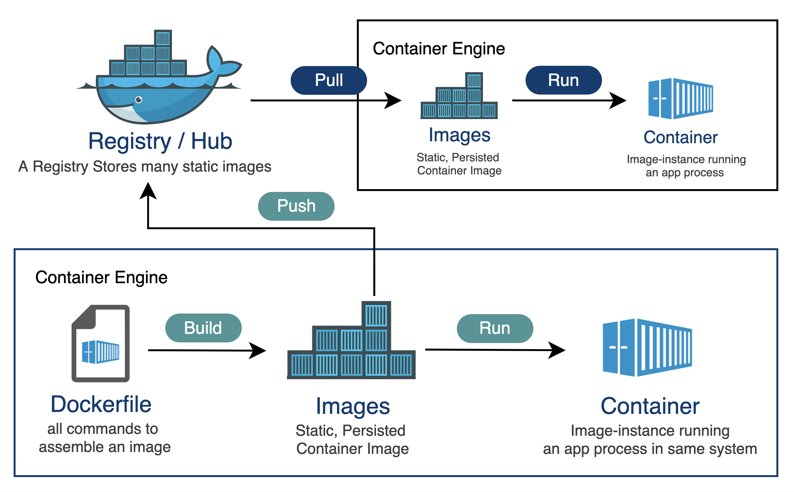
2.5.2 Image registry

An image registry is where images live so that other machines can pull them. Registries organize images into repositories, and identify image versions by a tag (for example myapp:1.4.2 or myapp:latest) and a digest.

The basic workflow is:

• We build an image,
• we tag it (for example myorg/api:1.2.3 or myorg/api:main),
• and we push it to a registry (Docker Hub, GHCR, ECR, GCR, and so on).

Then later, a server or a cluster pulls the image and runs it. Most of the time it pulls by tag, but we can also pull by digest. Note that tags are human-friendly labels and they can move over time (for example, :latest today is not the same as :latest next month). Digests are content-addressed hashes, so a digest uniquely identifies the exact image bytes.

Docker registry workflow.

Here is what that looks like with concrete commands:

# Build locally from a directory that contains a Dockerfile
docker build -t myapp:0.0.1 path/to/app

# Tag the same image for a registry/repository on GHCR
docker tag myapp:0.0.1 ghcr.io/myorg/myapp:0.0.1

# Push it
docker push ghcr.io/myorg/myapp:0.0.1

# Pull it somewhere else
docker pull ghcr.io/myorg/myapp:0.0.1

2.5.3 Running a container

Building an image creates an artifact; to use it, we need to run it. The relevant command is docker run, which (1) creates a container instance from an image and (2) starts it. If the image is not already present locally, Docker pulls it first.

Common docker run arguments include flags related to container lifecycle:

Flag	What it does	Example	Notes
--name NAME	Give the container a stable name	docker run --name web myapp:dev	Names make docker logs web and docker exec web ... easier.
--rm	Remove container on exit	docker run --rm myapp:dev	Automatically deletes the container when it exits; useful for keeping your system clean.
-d	Run in detached mode	docker run -d myapp:dev	Use docker logs to see output.
-it	Interactive + TTY	docker run -it ubuntu:24.04 bash	Useful for shells and debugging.
--restart POLICY	Restart behavior	docker run --restart unless-stopped myapp:dev	On a single host; orchestration platforms handle this differently.

Flags related to environment or settings inside the container:

Flag	What it does	Example	Notes
-e KEY=VAL	Set env vars	docker run -e MODE=dev myapp:dev	Prefer runtime injection for secrets.
--env-file FILE	Load env vars from a file	docker run --env-file .env myapp:dev	Convenient for local dev; treat files carefully if they contain secrets.
--workdir DIR	Set working directory	docker run --workdir /app myapp:dev	Overrides image WORKDIR.
--user UID:GID	Run as a specific user	docker run --user 1000:1000 myapp:dev	Useful when writing into mounted host directories.
--entrypoint CMD	Override entrypoint	docker run --entrypoint bash myapp:dev	Helpful for debugging images with strict entrypoints.

Flags related to network and network ports:

Flag	What it does	Example	Notes
-p HOST:CONTAINER	Publish a port	docker run -p 8080:8000 myapp:dev	Maps ports between host and container. From the outside, the service can be accessed on the HOST port; from inside the container, it appears as if it is on the CONTAINER port.
--network NET	Attach to a network	docker run --network mynet myapp:dev	Enables container-to-container communication via names on user-defined networks.

Flags related to storage and volumes:

Flag	What it does	Example	Notes
-v SRC:DST	Mount a volume or host path	docker run -v "$PWD":/app myapp:dev	Older syntax; see --mount for explicit forms.
--mount ...	Mount (explicit syntax)	docker run --mount type=bind,src=$PWD,dst=/app myapp:dev	Clearer for bind vs volume and extra options like read-only.

Flags related to configuring the compute capabilities of the container:

Flag	What it does	Example	Notes
--cpus N	CPU limit	docker run --cpus 2 myapp:dev	Local resource controls; enforced via cgroups.
-m MEM	Memory limit	docker run -m 4g myapp:dev	If set too low, your process may be OOM-killed.
--gpus ...	GPU access	docker run --gpus all myapp:dev	Requires NVIDIA container tooling on the host.
--shm-size SIZE	Shared memory size	docker run --shm-size 16G myapp:dev	Important for many ML/data workloads; increases /dev/shm beyond the small default.

Since we are going to run ML workloads inside containers: To access a host GPU inside a container, the container needs access to a host kernel driver. The container provides (or is given) the user-space libraries.

For NVIDIA GPUs, we need:

• NVIDIA GPU driver installed on the host (kernel driver + user-space driver components)
• NVIDIA Container Toolkit installed/configured for Docker (so Docker understands --gpus and can mount the right device nodes and driver libraries)
• and the --gpus ... flag is used to pass the GPUs to the container, e.g.

docker run --rm -it \
  --gpus all \
  --shm-size 16G \
  myapp:dev

For AMD GPUs (with ROCm), we need:

• AMDGPU kernel driver on the host
• DKMS packages (e.g., amdgpu-dkms) that build matching kernel modules for your running kernel
• pass the GPU with --device; /dev/kfd is the kernel interface ROCm uses for compute queues, and /dev/dri is used for GPU access
• and add the video and render groups so a non-root process in the container can access those devices

docker run --rm -it \
  --device=/dev/kfd --device=/dev/dri \
  --group-add video --group-add $(getent group | grep render | cut -d':' -f 3) \
  --shm-size 16G \
  myapp:dev

Once a container is running,

• docker ps lists running containers; add -a to include stopped containers (very useful when something starts and immediately exits)
• docker logs shows stdout/stderr from the container’s main process. The most useful forms are docker logs <container> for a snapshot, docker logs -f <container> to follow logs as they stream, docker logs --tail 200 <container> to see the most recent lines, and docker logs --since 10m <container> to focus on recent output.
• docker exec lets you run additional commands inside it (for example, opening a shell, running a one-off debug command, or checking a file). Common docker exec arguments:

Flag	What it does	Example	Notes
-it	Interactive + TTY	docker exec -it web bash	The most common pattern for debugging.
-u USER	Run as a user	docker exec -u root -it web bash	Useful when the container runs as non-root by default.
-w DIR	Set working directory	docker exec -w /app -it web bash	Mirrors --workdir for docker run.
-e KEY=VAL	Set env var for the exec’d process	docker exec -e DEBUG=1 web env	Affects only the one exec’d command, not the container’s base env.

TipA practical container debugging workflow

When a container “doesn’t work”, the fastest path is to narrow down what kind of failure it is: (1) it never started, (2) it started and immediately exited, (3) it is running but unhealthy, or (4) it is running but unreachable.

Typical sequence of checks:

1. Is it running?

   docker ps
   docker ps -a

   If it is not in docker ps but appears in docker ps -a, it exited.

2. What did it say before exiting? Check logs.

   docker logs <container>

   If the main process crashes during startup, the error message is usually here.

3. What metadata does the container engine have about it? (To inspect a container that has crashed, we should have run it without -rm.)

   docker inspect <container>

   This outputs detailed JSON about the container: its configuration (image, entrypoint, environment variables), its runtime state (running or stopped, exit code, last error), network settings (IP address, port mappings), volumes, and health status. Exit code 0 usually means “it finished successfully” (common when you accidentally run a one-off command instead of a long-lived service). Non-zero means a crash; the State.Error field often contains the last error message from the container runtime.

4. Try running it interactively. If it exits immediately, start a shell instead so you can inspect the environment.

   docker run --rm -it --entrypoint bash myapp:dev

   From inside the container, you can try starting the server manually and see errors directly.

5. If it is running, exec into it.

   docker exec -it <container> bash

   Common quick checks are: environment variables (env), config files, mounted paths, and whether the expected process is running.

6. If it is running but unreachable, check ports and binding. Did you publish the right container port? Is the app listening on 0.0.0.0 inside the container?

One subtle but important point: containers are designed around a “main” process. If that process exits, the container stops. Long-running services are usually started in the foreground (the process stays attached).

2.5.4 Overlay filesystem

We mentioned earlier that images are efficient because they are layered, so when building a container image, we can re-use common layers for different images. But the layered storage idea goes even further than this: when you run a container, those layers in the container image are mounted read-only, and the container gets a thin writable layer on top.

This means that we can run X instances of a container using image myapp, but:

• have only one copy of the myapp image, that all of the running instances share
• have only one copy of files like /bin/bash or /usr/lib/python3.11/... in RAM, even if many containers load them, since they come from the read-only shared layers
• while each container gets its own processes, its own heap/stack, and its own writable layer.

This in contrast to a VM scenario, where we would need X copies of all of those.

Most Linux container stacks implement this using a union filesystem, usually Linux overlayfs. The key behavior is copy-on-write (CoW): reads come from the shared read-only layers, and writes go into the container’s writable layer.

overlayfs conceptual view: lowerdir + upperdir -> merged mount

Here is how it works: it merges one or more read-only directories called lowerdir (these are the image layers), one writable directory called upperdir (this is the container’s writable layer), and an internal workdir.

Applications see a single merged filesystem, but physically if a file is never modified it is served directly from the lowerdir, while on the first write to a file that exists in a lowerdir overlayfs performs a copy-up into the upperdir and then applies the write there.

Deletions are special: if you delete a file that exists in a lowerdir, overlayfs creates a whiteout entry in the upperdir so the file disappears from the merged view even though the bytes still exist in the lower layers. Similarly, entire directories can be marked as an opaque directory.

The writable layer is also why containers are ephemeral. If you write user uploads, logs, or model artifacts into the container filesystem, that data disappears when the container is deleted, because that writable layer does not persist. Persistent data should live outside the container filesystem, typically via a volume or an external service (database, object store). For local development, you often use a bind mount to share code or data with a container.

2.5.5 Container networking

Container networking is easiest to understand if we treat a container like a tiny host that “lives” inside another host. In fact, Docker gives each container its own network namespace, which means the container has its own virtual “interfaces”.

The figure below shows the common default setup (“bridge mode”). Every container is connected to a virtual switch on the host. Concretely, Docker creates a host-side Linux bridge (often called docker0) and plugs each container into that bridge using a veth pair. One end of the veth pair looks like a NIC inside the container, and the other end is attached to the bridge on the host. At this point, container-to-container traffic on the same bridge looks like normal LAN traffic: packets go from one container NIC to the bridge and then to another container NIC.

Container networking (bridge mode): namespaces, veth pairs, and docker0

The bridge network is usually a private IP range that only exists on the host. When a container needs to reach the Internet (for example, pip install or downloading data), the host acts like the router/NAT gateway we discussed in the Network section. Docker sets up SNAT rules on the host so outbound traffic from container private IPs is rewritten to the host’s IP, and replies can be translated back and forwarded to the right container.

The most common inbound operation is port mapping:

docker run --rm -p 8080:8000 myapp:dev

This is the same idea as DNAT from the Network section, but on a single machine. Docker installs rules so traffic sent to the host on port 8080 is rewritten and forwarded to the container’s private IP on port 8000.

There are a few common conceptual pitfalls:

• Inside a container, localhost means the container itself, not the host and not another container.
• On a cloud VM, publishing a port is not the only step. The cloud security group still controls whether the Internet can reach that host port.

2.6 Container orchestration

Once you can package an app as an image, the next problem is operational: you rarely run just one container, and you rarely want to babysit them. You need a consistent way to start the right set of containers with the right configuration, restart them when they crash, update them without downtime (or with controlled downtime), connect them together (networking and service discovery), enforce resource boundaries (limits), and place workloads where they belong (for example, GPU jobs on GPU nodes).

This is what container orchestration provides.

We will describe two frameworks:

• Docker compose
• Kubernetes (often abbreviated as “K8S”)

2.6.1 Docker compose

Docker Compose is the smallest step up from docker run. It helps you orchestrate multiple containers on one host: you declare what you want in a compose.yaml, then run it with docker compose up.

Under the hood it still creates normal containers, networks, and volumes. The main difference is that Compose gives you a way to define a multi-container app, predictable naming and a shared default network, and a workflow for bringing the whole app up/down.

For example here is a single-service compose.yaml for a small web API:

services:
  api:
    build: .
    ports:
      - "8080:8000"
    environment:
      LOG_LEVEL: "info"
    command: ["uvicorn", "app:app", "--host", "0.0.0.0", "--port", "8000"]

Conceptually, this is the same as running:

docker build -t api:dev .
docker run --rm -p 8080:8000 -e LOG_LEVEL=info api:dev \
  uvicorn app:app --host 0.0.0.0 --port 8000

In other words, we have moved the “knobs” from CLI flags into YAML.

Many of the things you do with docker run have direct counterparts in Compose:

docker run concept	Compose field	Example
Image	image	image: nginx:1.27
Build from Dockerfile	build	build: .
Override command	command	command: ["python", "app.py"]
Publish ports	ports	ports: ["8080:8000"]
Environment vars	environment	environment: { MODE: "dev" }
Env file	env_file	env_file: [".env"]
Mount volume/bind	volumes	volumes: ["./src:/app"]
Working directory	working_dir	working_dir: /app
Run as user	user	user: "1000:1000"
Restart policy	restart	restart: unless-stopped
Attach to a network	networks	networks: ["appnet"]
Increase shared memory	shm_size	shm_size: "16g"

Some CLI flags are workflow-specific rather than configuration-specific. The --rm flag is a runtime choice; Compose supports it for one-off runs: docker compose run --rm api .... The -d flag maps to how you invoke Compose: docker compose up -d.

But, besides for running containers with various flags, we can also do new things!

An .env file placed in the same directory is read by Compose itself and can be used for variable interpolation in the YAML.

For example:

services:
  api:
    image: myorg/api:${TAG}
    ports:
      - "${HOST_PORT}:8000"
    environment:
      DATABASE_URL: "${DATABASE_URL}"

and a matching .env:

TAG=dev
HOST_PORT=8080
DATABASE_URL=postgresql://postgres:example@db:5432/postgres

This pattern lets you keep a single Compose file and swap settings in different environments without editing YAML. Instead of a .env file, you could also set env vars for Compose in the shell right before the command:

TAG=dev HOST_PORT=8080 DATABASE_URL=postgresql://postgres:example@db:5432/postgres \
  docker compose up

Compose can also encode extra behavior that is awkward to express with docker run alone. For example, you can define a healthcheck:

services:
  api:
    build: .
    ports:
      - "8080:8000"
    healthcheck:
      test: ["CMD", "curl", "-fsS", "http://localhost:8000/healthz"]
      interval: 5s
      timeout: 2s
      retries: 10
      start_period: 10s

Health checks are useful when one service depends on another, and you only want to start a service when its dependencies are ready to use. Compose lets you express this with depends_on:

services:
  api:
    build: .
    depends_on:
      db:
        condition: service_healthy

  db:
    image: postgres:16
    environment:
      POSTGRES_PASSWORD: example
    healthcheck:
      test: ["CMD-SHELL", "pg_isready -U postgres"]
      interval: 5s
      timeout: 3s
      retries: 10

This makes it much easier to start up groups of services in sequence.

Compose makes it easy to model storage and connectivity explicitly. A named volume is separate from any particular container instance. If you run docker compose down and then later docker compose up again, Compose will recreate the containers but reattach the same named volume by default, so your database files (or other state) are still there. (You have to explicitly remove volumes, for example with docker compose down -v, to throw that state away.)

services:
  api:
    build: .
    ports:
      - "8080:8000"
    environment:
      DATABASE_URL: "postgresql://postgres:example@db:5432/postgres"
    depends_on:
      db:
        condition: service_healthy

  db:
    image: postgres:16
    environment:
      POSTGRES_PASSWORD: example
    volumes:
      - db_data:/var/lib/postgresql/data
    healthcheck:
      test: ["CMD-SHELL", "pg_isready -U postgres"]
      interval: 5s
      timeout: 3s
      retries: 10

volumes:
  db_data:

Notice db is used as a hostname (db:5432). In Compose, networking is modeled as one or more named networks (think: virtual switches). By default, Compose creates one private bridge network for the project and attaches every service to it, giving each container an IP address on that network. Compose also sets up DNS on that network so the service name becomes the hostname, which is why db:5432 works without us manually assigning IP addresses.

We can also define and name networks explicitly. This is useful when we want multiple networks, or when we want stable, human-chosen network names:

services:
  web:
    image: myorg/web:dev
    ports:
      - "8080:8000"
    networks:
      - frontend
      - backend

  db:
    image: postgres:16
    environment:
      POSTGRES_PASSWORD: example
    networks:
      - backend

networks:
  frontend:
    name: myapp-frontend
  backend:
    name: myapp-backend

In this example, web is connected to two networks, while db is only connected to backend. That means web can talk to db (they share a network), but containers that are only on frontend cannot reach db directly. The name: fields set the actual Docker network names, instead of letting Compose generate a default name like myproject_default.

Docker compose is also helpful for sidecars and run-to-completion services. In real systems, not every container is a long-running server. One common pattern is a sidecar: it is a separate container that shares a network (and sometimes volumes) with the main service. For example, we might run a small helper container that reads environment variables and writes an application config file into a shared volume. The main service then reads that config file at startup.

Another common pattern is an init container-style service: it runs a one-time setup step (for example, creating database tables or running a migration), and then it exits.

Compose does not have a special “init container” object, but you can model it by defining a service that runs a setup command and is meant to exit:

services:
  migrate:
    build: .
    command: ["python", "-m", "alembic", "upgrade", "head"]
    environment:
      DATABASE_URL: "postgresql://postgres:example@db:5432/postgres"
    depends_on:
      db:
        condition: service_healthy
    restart: "no"
    profiles: ["init"]

The same idea shows up in a few other “pattern” containers you will see in practice.

Compose really shines when you need a system of containers, rather than a single container. For example, suppose we want to run a web service + database + background worker:

services:
  web:
    build: .
    ports:
      - "8080:8000"
    environment:
      DATABASE_URL: "postgresql://postgres:example@db:5432/postgres"

  worker:
    build: .
    command: ["python", "worker.py"]
    environment:
      DATABASE_URL: "postgresql://postgres:example@db:5432/postgres"
    depends_on:
      db:
        condition: service_healthy

  db:
    image: postgres:16
    environment:
      POSTGRES_PASSWORD: example
    volumes:
      - db_data:/var/lib/postgresql/data
    healthcheck:
      test: ["CMD-SHELL", "pg_isready -U postgres"]
      interval: 5s
      timeout: 3s
      retries: 10

volumes:
  db_data:

All three services are connected to the same user-defined network (Compose creates one by default for the project), so web can connect to db at hostname db, worker can connect to db at hostname db, and web and worker can also reach each other by service name if you expose endpoints internally. That “connect by name” behavior is the foundation of container service discovery.

TipDebugging with Compose

When something goes wrong in a Compose stack, the debugging workflow is similar to single-container Docker, but we work across multiple services at once.

Start by checking what is running and what is not:

docker compose ps

This shows the state of each service (running, exited, restarting). If a service exited, look at its logs:

docker compose logs <service>
docker compose logs -f <service>   # follow/stream logs

For a shell inside a running container:

docker compose exec <service> bash

If the container is not running (crashed on startup), we can start a one-off container in the same network with an interactive shell:

docker compose run --rm <service> bash

A common pattern is to run a “debug” container that shares the network with the rest of the stack, so we can test connectivity (can we reach db? can we curl web?). We can also add a lightweight utility service to the compose.yaml for this purpose.

Most Compose debugging reduces to the same root causes as single-container Docker: wrong command/entrypoint, missing or incorrect environment variables, a dependency not ready (use depends_on with health checks), or networking misconfiguration (wrong service name, port not exposed).

2.6.2 Kubernetes

When your workload outgrows a single machine, you need orchestration across multiple hosts. That changes the problem: now you need a control plane that can decide where a container should run, keep it running, and move it if the underlying machine fails.

Kubernetes (K8s) is the dominant system for this. Its core promise is: you declare the desired state (“run 3 replicas of this service”), and Kubernetes makes the state of the cluster match your declaration.

To talk about Kubernetes clearly, we need a bit of vocabulary:

• A node is a machine in the cluster that runs work.
• A pod is the unit that Kubernetes schedules onto a node; it usually contains one main container (and sometimes helper containers).
• A replica is one copy of a pod, and we often run multiple replicas of a service.
• A Deployment (or, for stateful workloads, a StatefulSet) is the object that manages those replicas over time: it creates them, replicates them, replaces them when they die, and rolls them forward when we update the spec.
• A Service gives us a stable name and endpoint that routes traffic to the right pods.
• Finally, a manifest is the YAML we submit to Kubernetes that defines these objects.

Kubernetes runs on a cluster, which is just a group of machines. The machines that actually run our containers are the nodes. When we submit work, Kubernetes picks a node for it. That decision is made by the scheduler.

Kubernetes cluster architecture: control plane decides what should exist, worker nodes run workloads

The use of a scheduler forces us to be explicit about resources. We have to tell it how much CPU and memory a pod should get, using requests and limits. Requests are what the scheduler uses to decide where something can fit. Limits are caps which are actually enforced at runtime.

Pod placement is based on requests: the scheduler finds a node where requested CPU/memory fit

If requests are too high, the scheduler may never place the pod (it will sit in Pending). If memory is limited too tightly, the process can be killed when it exceeds the cap (you will often see OOMKilled). As a rule of thumb, we set requests based on what we need to run reliably, and we only set tight limits when we have a clear reason to cap a workload.

Rightsizing requests and limits: under-request hurts reliability, over-request wastes capacity

GPUs work the same way, except we request a discrete device count instead of a fraction of CPU. In a pod manifest we can ask for (say) one NVIDIA GPU, and the scheduler will only place that pod on a node that actually has a free GPU,. Kubernetes relies on a GPU device plugin on the node to make the GPU visible inside the container.

Kubernetes does not schedule individual containers; it schedules pods. A pod is the “thing that runs”: it gets an IP address, it can mount volumes, and Kubernetes moves it around as a unit. Most pods contain one main container, but a pod can also include helper containers that should live right next to the main one.

Kubernetes also needs a way to tell whether a pod is healthy and whether it is ready to receive traffic. That is what probes are for. A liveness probe is a basic “is it still alive?” check. A readiness probe is a “is it ready to serve?” check. A startup probe is a “give it time to start” check for slow bootstraps. Readiness matters a lot during updates, because it controls when new pods start receiving traffic.

The diagram below shows the main pod lifecycle we will see. The happy path goes straight down the middle: we apply a manifest, the pod is Pending while Kubernetes is waiting to schedule it, it moves to ContainerCreating once a node has been chosen, it becomes Running when the container starts, and it becomes Ready only after the readiness check passes. (Ready is not itself a state - the state stays as Running but with a readiness indicator.) Finally, some workloads end on purpose (for example batch jobs), and show up as Completed when the process exits successfully.

Off to the side are common ways the happy path can get interrupted. A pod can stay Pending if no node fits. It can fail when pulling the image, mounting volumes, or setting up networking - for example, if the image pull fails we may see ErrImagePull and then ImagePullBackOff as it keeps retrying and failing. If a container crashes repeatedly whenever it starts, we may see CrashLoopBackOff.

We usually wrap pods in a Deployment. A Deployment keeps the right number of replicas running. If a pod dies, it makes a new one. If we change the image tag, it rolls out the new version.

Let’s see some specific examples. In our course, the Kubernetes YAML we write is mostly a few kinds of objects. The most common one is a Deployment plus a Service. Here is a simple pair (similar to what you will see in the labs):

apiVersion: apps/v1
kind: Deployment
metadata:
  name: myapp
  namespace: myapp-staging
spec:
  replicas: 2
  selector:
    matchLabels:
      app: myapp
  template:
    metadata:
      labels:
        app: myapp
    spec:
      containers:
        - name: myapp
          image: ghcr.io/myorg/myapp:0.0.1
          ports:
            - containerPort: 8000
          resources:
            requests:
              cpu: "250m"
              memory: "256Mi"
            limits:
              cpu: "1"
              memory: "512Mi"
---
apiVersion: v1
kind: Service
metadata:
  name: myapp
  namespace: myapp-staging
spec:
  selector:
    app: myapp
  ports:
    - port: 80
      targetPort: 8000
  externalIPs:
    - 129.114.25.1

The Deployment part is the “run N copies of this container” piece. The Service part is the “give it a stable name and a stable port” piece. Notice that the Service forwards to pods by label (app: myapp).

By default, a Service is a ClusterIP Service, which means it is only reachable inside the cluster. In that default setup, other pods can reach it by name (for example http://myapp:80). That request hits the Service on port 80 (port: 80), and the Service forwards it to the pods on port 8000 (targetPort: 8000). Nothing outside the cluster can reach it. In our environment, we will often keep the Service as ClusterIP but add public externalIPs so it is reachable from outside. That is what the example above is doing: traffic sent to 129.114.25.1:80 is accepted by the cluster and forwarded to the Service port 80, and then forwarded again to the pods on port 8000.

There are two other common ways to expose a Service:

• NodePort: Kubernetes opens a port on every node. Traffic to <node-ip>:<nodePort> is forwarded to the Service port, and then forwarded to the pods targetPort. For our myapp Service, this would mean: <node-ip>:30080 -> Service port 80 -> pod port 8000. It would look like:

  apiVersion: v1
  kind: Service
  metadata:
    name: myapp
    namespace: myapp-staging
  spec:
    type: NodePort
    selector:
      app: myapp
    ports:
      - port: 80
        targetPort: 8000
        nodePort: 30080

• LoadBalancer: on managed cloud Kubernetes, Kubernetes can ask the cloud provider to create a load balancer for us, and that load balancer gets a public IP. Conceptually, traffic to <lb-ip>:80 is forwarded to the Service port 80, and then forwarded to the pods on port 8000. For myapp, it would look like:

  apiVersion: v1
  kind: Service
  metadata:
    name: myapp
    namespace: myapp-staging
  spec:
    type: LoadBalancer
    selector:
      app: myapp
    ports:
      - port: 80
        targetPort: 8000

That takes care of networking with the outside world! For networking between pods, Kubernetes provides DNS-based service discovery: pods can reach a Service by its name within the same namespace (e.g., http://myapp:80) or across namespaces (e.g., http://myapp.myapp-staging:80). The Service acts as a stable virtual IP that routes to the underlying pods, so individual pod IPs can change without breaking inter-pod communication.

Next, let’s think about storage. Stateful services need storage that outlives pods. In Kubernetes we usually start with a PersistentVolumeClaim (PVC) and then mount it into a Deployment:

apiVersion: v1
kind: PersistentVolumeClaim
metadata:
  name: postgres-pvc
  namespace: myapp-platform
spec:
  accessModes:
    - ReadWriteOnce
  resources:
    requests:
      storage: 5Gi
---
apiVersion: apps/v1
kind: Deployment
metadata:
  name: postgres
  namespace: myapp-platform
spec:
  replicas: 1
  selector:
    matchLabels:
      app: postgres
  template:
    metadata:
      labels:
        app: postgres
    spec:
      containers:
        - name: postgres
          image: postgres:16
          env:
            - name: POSTGRES_PASSWORD
              valueFrom:
                secretKeyRef:
                  name: postgres-credentials
                  key: password
          volumeMounts:
            - name: data
              mountPath: /var/lib/postgresql/data
      volumes:
        - name: data
          persistentVolumeClaim:
            claimName: postgres-pvc

How does that PVC turn into a real, durable disk? Kubernetes binds a PVC to a PersistentVolume (PV). In most managed clusters, we do not create PVs by hand. Instead, the cluster has a StorageClass backed by a storage driver, so when we create the PVC Kubernetes can dynamically provision a block storage volume in the provider. If we are managing storage by hand (for example, in a bare metal cluster or a minimal on-prem setup), we may need to pre-provision the disk ourselves and create a PV resource that points to it, and only then will our PVC bind to that PV.

Finally, some work is meant to run and then exit. That is what a Job is for. For example, we might run a one-time setup command after the cluster is up:

apiVersion: batch/v1
kind: Job
metadata:
  name: setup
  namespace: myapp-platform
spec:
  backoffLimit: 3
  template:
    spec:
      restartPolicy: OnFailure
      containers:
        - name: setup
          image: alpine:3.20
          command: ["sh", "-c"]
          args:
            - echo "hello from setup"

Raw YAML can get repetitive when we have multiple environments (staging vs production) and many services. We can use Helm or similar systems to keep one set of templates and swap environment-specific values (replica count, image tags, external IPs), like we did with Docker Compose and .env.

Another way to reduce repetition is to separate configuration from workloads. A ConfigMap lets us store settings (for example, feature flags, file paths, or a service URL) once and then inject them into many pods, instead of duplicating the same values across multiple Deployment manifests.

Once we put it all together, the workflow is pretty simple. We write YAML manifests (Deployments, Services, Jobs), and we apply them to the cluster:

kubectl apply -f k8s/
kubectl get pods
kubectl describe pod <pod>
kubectl logs <pod>

Manifests often contain multiple objects separated by --- (for example, a Service + a Deployment in one file). Applying the file creates or updates all of them in one shot.

TipDebugging Kubernetes (quick path)

When a pod is not behaving, it helps to ask one question first: is it stuck before it starts, or did it start and then fail?

If the pod never got scheduled (it sits in Pending), Kubernetes could not find a node that fits. Start here:

kubectl describe pod <pod>

The “Events” section usually tells us why, in plain terms (not enough CPU, not enough memory, or a placement rule that no node satisfies).

If the pod was scheduled but the container is not running (statuses like CrashLoopBackOff, Error, or ImagePullBackOff), check logs and then describe:

kubectl logs <pod>
kubectl logs <pod> --previous   # logs from the last crashed instance
kubectl describe pod <pod>

ImagePullBackOff usually means Kubernetes cannot pull the image (wrong name, missing credentials, or the registry is unreachable). CrashLoopBackOff usually means the process starts and then exits; the logs typically show the real error.

If the pod is running but the app is unhealthy or unreachable, check whether it is passing probes and whether the Service is actually routing to it:

kubectl get endpoints <service>
kubectl describe service <service>

If the endpoints list is empty, the Service is not seeing any ready pods that match its selector. We can also open a shell inside the pod to test from the inside:

kubectl exec -it <pod> -- bash

For network debugging, it is often useful to run a temporary “debug” pod in the same namespace and test DNS and connectivity:

kubectl run debug --rm -it --image=busybox -- sh

From there we can nslookup <service>, wget, or nc to test connectivity.

When we are done, we usually clean up by deleting the manifests we applied:

kubectl delete -f k8s/

Once our app is running and we can debug it, the next question is scaling. In Kubernetes, scaling usually happens at two levels.

First, we can scale the number of pods for a service. A Horizontal Pod Autoscaler (HPA) can increase or decrease the replica count of a Deployment based on metrics. Here is a minimal HPA that targets the myapp Deployment and keeps it between 2 and 6 replicas based on CPU:

apiVersion: autoscaling/v2
kind: HorizontalPodAutoscaler
metadata:
  name: myapp-hpa
  namespace: myapp-staging
spec:
  scaleTargetRef:
    apiVersion: apps/v1
    kind: Deployment
    name: myapp
  minReplicas: 2
  maxReplicas: 6
  metrics:
    - type: Resource
      resource:
        name: cpu
        target:
          type: Utilization
          averageUtilization: 50

In practice, HPA needs a way to measure CPU and memory. Many clusters install a metrics server for this. Also, CPU utilization for HPA is usually computed relative to CPU requests, so if we do not set reasonable requests, the autoscaling behavior becomes hard to interpret.

Second, in a managed Kubernetes environment, we can scale the cluster itself. A cluster autoscaler adds or removes nodes. This kicks in when there is not enough capacity to place pods at all (pods sit in Pending because no node fits). The key difference is: HPA changes how many pods we want, while cluster autoscaling changes how many machines we have to run them.

2.7 Comparison

The table below summarizes how the same ideas show up in three places: docker run (one container on one host), Docker Compose (many containers on one host), and Kubernetes (many pods across many hosts).

Concept	docker run	Docker Compose	Kubernetes
Image	IMAGE[:TAG]	image (in service definition)	image (in container spec)
Build from Dockerfile	docker build ...	build (in service definition)	Build/push image separately, then set image
Command / entrypoint	--entrypoint ... + trailing args	entrypoint / command (in service definition)	command / args (in container spec)
Environment variables	-e KEY=VALUE --env-file	environment / env_file (in service definition)	env (often from ConfigMaps/Secrets)
Ports (inbound)	-p HOST:CONTAINER	ports (in service definition)	Service ports: port -> targetPort (and type)
Volumes / storage	-v host:container or named volume	volumes (in service definition)	volumeMounts + volumes (often via PVC/PV)
Network attachment	--network <net>	networks (service + top-level)	Pod network + Services (plus VPC rules)
Restart on failure	--restart ...	restart (in service definition)	Deployment/Job controller + kubelet restarts containers
Health checks	--health-cmd ... (and timing flags)	healthcheck (in service definition)	Probes: livenessProbe readinessProbe startupProbe
CPU / memory	--cpus ... --memory ...	deploy.resources (limited support)	resources.requests resources.limits
NVIDIA GPU	--gpus ...	deploy.resources. reservations.devices (driver nvidia)	resources.limits. nvidia.com/gpu: 1
AMD GPU	--device ... (ROCm devices)	devices (in service definition)	resources.limits. amd.com/gpu: 1
Scaling (replicas)	Start more containers manually (no load balancing)	docker compose up --scale web=3 (no load balancing)	Deployment spec.replicas
Autoscaling	N/A	N/A	HPA + cluster autoscaler

2.8 Key terms

• base image: The starting image that your image builds on top of (runtime or distro base).
• Bastion (jump host): A small public VM used as the only administrative entry point to a private network. Also called a jump host.
• bind mount: Mounting a host filesystem path into a container.
• boot volume: The disk an instance boots from; contains OS and base software.
• build cache: Saved results of prior build steps reused when inputs haven’t changed.
• build context: The directory of files sent to the Docker engine for use by COPY/ADD during a build.
• CaaS: Container as a Service: a managed platform for running containers (scheduling, service discovery, basic lifecycle), often built around Kubernetes or a similar orchestrator.
• cache invalidation: When a change to an input causes a cached build step (and all following steps) to be rebuilt.
• cluster: A set of machines managed together by Kubernetes: control plane + worker nodes.
• cluster autoscaler: A component that adjusts the number of cluster nodes based on pending pods and capacity; separate from pod autoscaling.
• ClusterIP: A Service type reachable only inside the cluster via a virtual IP and DNS name.
• ConfigMap: A Kubernetes object that stores non-secret configuration data (key/value pairs) that pods can consume as environment variables or mounted files.
• container: An isolated process (or set of processes) running on a shared host OS using kernel features like namespaces and cgroups.
• container engine: Software that runs and manages containers on a host, providing isolation and resource controls (for example Docker Engine or containerd).
• container image: A packaged filesystem + metadata describing how to run an app (entrypoint, env, exposed ports), typically conforming to the OCI image spec.
• container orchestration: Coordinating and managing the lifecycle of many containers: scheduling, scaling, restarts, updates, and connectivity.
• copy-on-write: Copy-on-write: data is shared until a write occurs, at which point a private copy is created.
• copy-up: The operation where overlayfs copies a file from the lowerdir into the upperdir before modifying it.
• data volume: A non-bootable disk attached to an instance for persistent state; you format/mount it inside the OS.
• depends_on: A Compose setting that declares a service dependency (and optionally gates startup on a condition like the dependency being healthy).
• Deployment: A Kubernetes workload object that manages a set of identical pods and supports rolling updates.
• detached mode: Run a container in the background; the command still runs, but the CLI returns immediately.
• digest: A content-addressed identifier (sha256…) for an image manifest; changing image content changes the digest.
• DNAT: Destination Network Address Translation: rewrites the destination IP (and sometimes destination port) so inbound traffic to a public endpoint is delivered to a private instance/service.
• Docker Compose: A tool and file format for defining and running multi-container applications: you declare services, networks, and volumes in YAML, and Compose runs the corresponding containers.
• Dockerfile: A build recipe for container images, most commonly used by Docker-compatible builders.
• Ephemeral storage: Storage that is tied to the lifetime of an instance; data is lost when the instance is terminated or rebuilt.
• FaaS: Function as a Service: you deploy individual functions that run on demand (HTTP/event) and the platform scales them automatically.
• healthcheck: A periodic check the container runtime runs to determine whether a service is healthy (distinct from ‘container is running’).
• Helm: A Kubernetes packaging and templating system: Helm charts define parameterized Kubernetes resources, installed as releases.
• Horizontal Pod Autoscaler (HPA): Horizontal Pod Autoscaler: automatically adjusts the number of pod replicas for a workload based on metrics (often CPU utilization).
• hypervisor: Virtual machine monitor: the software layer that creates and runs virtual machines by multiplexing physical hardware (CPU, memory, devices) across isolated guest OS instances.
• IaaS: Infrastructure as a Service: the provider offers virtualized compute, networking, and storage primitives (instances, volumes, IPs, networks).
• image registry: A service that stores and distributes container images (e.g., Docker Hub, ECR, GCR, ACR).
• init container: A short-lived container that performs setup work (migrations, schema creation, downloading artifacts) and then exits; the system should still be correct if it is re-run.
• instance: A provisioned unit of compute capacity (a VM, container, or bare-metal server) created from a template/configuration and treated as a replaceable resource.
• Job: A Kubernetes workload object that runs a pod to completion (optionally many times); used for batch tasks like training or one-time setup.
• Kubernetes (K8s): Kubernetes: a container orchestration system that schedules and manages containers (as pods) across a cluster of machines.
• limits: Resource limits: hard caps on CPU/memory/etc; enforced by the runtime/cgroups to prevent noisy neighbors.
• liveness probe: A health check that determines whether a container should be restarted; failing it triggers a restart.
• LoadBalancer: A Service type exposed via an external load balancer (cloud-integrated).
• lowerdir: The read-only directories that make up the base of the merged view (typically the image layers).
• managed services: Cloud services where the provider operates and maintains the underlying software (databases, caches, queues, storage) so we consume them via API rather than running them ourselves.
• manifest: A YAML file that declares Kubernetes resources and their desired configuration.
• metrics server: A Kubernetes addon that provides resource metrics (CPU/memory) to the HPA and to kubectl top.
• network interface cards (NICs): Network interface card: the hardware (or virtual device) that attaches a host to a network. A VM typically has virtual NICs backed by a physical NIC on the host machine.
• network namespace: An isolated network stack (interfaces, routes, ports) provided by the Linux kernel.
• node: A machine (VM or bare metal) that runs Kubernetes workloads.
• NodePort: A Service type that exposes the Service on a port on every node (nodeIP:nodePort).
• nodes: A machine (VM or bare metal) that runs Kubernetes workloads.
• opaque directory: A marker that hides a directory’s contents from lower layers, making the upper directory appear to replace it.
• overlayfs: The Linux implementation commonly used for container image layering (often via the overlay2 storage driver).
• PaaS: Platform as a Service: a managed application hosting platform where you deploy app code (or an app image) and the provider operates most of the runtime and infrastructure.
• persistent volume: A durable block device provided by the cloud that can be attached/detached from instances and survives instance replacement.
• PersistentVolume (PV): A cluster resource that represents a piece of storage (often a disk) that can be mounted by pods.
• PersistentVolumeClaim (PVC): A claim for storage by a pod; it requests size and access mode and is bound to a PersistentVolume.
• pod: The basic unit of execution in Kubernetes: one or more containers that share a network namespace and are scheduled together.
• port mapping: Publishing a container port to the host by mapping host_port:container_port.
• Private cluster with a head node: A set of private instances that can communicate with each other freely for internal coordination and data exchange.
• private IP addresses: An IP address used only inside a private network; not globally routable on the public internet.
• public IP addresses: A globally routable IP address reachable from the public internet (subject to firewall rules).
• readiness probe: A health check that determines whether a pod is ready to receive traffic; failing it removes the pod from service endpoints.
• replica: One copy of a pod; Kubernetes can run many replicas for scaling and high availability.
• repositories: A named collection of images, typically referenced as registry/namespace/name.
• requests: Resource requests: the amount of CPU/memory/etc a pod asks for; used for scheduling decisions.
• SaaS: Software as a Service: a complete application delivered over the network; you consume it rather than deploying code to it.
• scheduler: The component that decides which node should run each pod based on resource requests, constraints, and policies.
• security groups: Cloud-managed firewall policy that allows or denies traffic based on direction, protocol, ports, and peers; typically attached to an instance or network interface.
• Service: A stable network endpoint (virtual IP + DNS name) that routes traffic to a set of pods.
• service discovery: Mechanisms that let services find each other by stable names rather than hard-coded IP addresses.
• sidecar: A helper container that runs alongside a main service to provide a supporting capability (proxying, logging, metrics, cert management) without changing the main container image.
• source NAT (SNAT): Source Network Address Translation: rewriting the source IP (and often the source port) of outbound traffic so private hosts can access the public internet.
• startup probe: A probe used during slow startups; until it succeeds, liveness/readiness are deferred to avoid premature restarts.
• StatefulSet: A Kubernetes workload object like a Deployment but with stable identities and stable storage; commonly used for databases.
• StorageClass: A policy that tells Kubernetes what kind of storage to provision for a PVC (e.g., which cloud disk type) and how.
• tag: A human-friendly label (often version-like) that points to an image; tags are typically mutable.
• Three-tier networks: A common cloud network layout that uses separate networks to isolate the frontend, application logic, and data.
• type 1 hypervisor: Bare-metal hypervisor: a hypervisor that runs directly on server hardware (or is integrated into the host kernel) and provides VM isolation as a core function.
• type 2 hypervisor: Hosted hypervisor: a hypervisor that runs as an application on top of a normal host OS.
• union filesystem: A filesystem that merges multiple directories (layers) into a single view, commonly implemented with overlayfs on Linux.
• upperdir: The writable directory for a specific container; all file changes go here.
• variable interpolation: Replacing variables in configuration files with values from an environment or .env file, usually written as ${VAR}.
• veth pair: Virtual Ethernet pair: two linked virtual interfaces; one end in the container namespace, one on the host.
• virtual machines (VMs): A virtual machine: an emulated computer with its own guest OS running on a hypervisor.
• volume: A mechanism to persist data outside a container’s writable layer (e.g., Docker volumes or Kubernetes persistent volumes).
• VPC: Virtual Private Cloud: a logically isolated virtual network with our own IP ranges, routing, and security rules.
• whiteout: A marker that hides a file from lower layers in the merged view; used to represent deletions.
• workdir: A scratch directory overlayfs uses for bookkeeping during operations like renames and copy-up.

---

1. Peter Mell and Tim Grance, “The NIST Definition of Cloud Computing,” NIST Special Publication 800-145, September 2011. https://doi.org/10.6028/NIST.SP.800-145